Writing reliable and maintainable code is a fundamental part of software
development, and unit testing is one of the most effective ways to ensure your
code works as expected. Unit tests help catch bugs early, ensure that changes to
the codebase don’t introduce new issues, and serve as a form of documentation
for your code’s expected behavior.
In this article, we’ll explore how to set up and use Google Test (also known as
googletest), a popular C++ testing framework, to test your C and C++ code. We’ll
walk through the installation process, demonstrate basic assertions, and then
dive into testing a more complex feature—the variant data type.
Installation and Setup
Google Test makes it easy to write and run unit tests. It integrates well with
build systems like CMake, making it straightforward to include in your project.
Let’s go step-by-step through the process of installing and setting up Google Test
in a CMake-based project.
Step 1: Add Google Test to Your Project
First, we need to download and include Google Test in the project. One of the easiest
ways to do this is by adding Google Test as a subdirectory in your project’s
source code. You can download the source directly from the Google Test GitHub repository.
Once you have the source, place it in a lib/ directory within your project.
Your directory structure should look something like this:
Now that you have Google Test in your project, let’s modify your CMakeLists.txt
file to integrate it. Below is an example of a CMake configuration that sets up
Google Test and links it to your test suite:
project(tests)

# Add Google Test as a subdirectory
add_subdirectory(lib/googletest-1.14.0)

# Include directories for Google Test and your source files
include_directories(${gtest_SOURCE_DIR}/include ${gtest_SOURCE_DIR})
include_directories(../src)

# Add the executable that will run the tests
add_executable(Google_Tests_run
src/tests1.cpp
src/tests2.cpp
src/tests3.cpp)

# Link the Google Test library and any other necessary libraries
target_link_libraries(Google_Tests_run gtest gtest_main myproject)
This CMake setup includes Google Test in your project by adding it as a
subdirectory, and it links your test suite to the gtest and gtest_main
libraries. Now you’re ready to write and run unit tests!
Step 3: Build and Run the Tests
To compile the tests, simply run the following commands from the root of your project directory:
mkdir build
cd build
cmake ..
make
Once the build is complete, you can run your tests with:
./Google_Tests_run
This command will execute all the tests defined in your test files. Now that the
environment is set up, let’s move on to writing some unit tests using Google Test.
Basic Assertions with Google Test
Before diving into testing our variant data type, let’s explore some of the basic
assertions provided by Google Test. Assertions are used to check that a
particular condition holds true during test execution. If the condition is false,
the test fails.
Common Assertions
Here are some of the most commonly used assertions:
EXPECT_EQ(val1, val2): Checks that val1 is equal to val2.
EXPECT_NE(val1, val2): Checks that val1 is not equal to val2.
EXPECT_TRUE(condition): Checks that the condition is true.
EXPECT_FALSE(condition): Checks that the condition is false.
ASSERT_EQ(val1, val2): Like EXPECT_EQ, but if the assertion fails, it aborts the current function.
Let’s look at a simple example that tests basic operations:
When you run this test, Google Test will evaluate each assertion and output the
result. If any assertion fails, it will print a detailed message showing the
expected and actual values.
Now that you’ve seen how to use basic assertions, let’s move on to testing a more
complex feature: the variant data type.
Testing the Variant Data Type
In a previous post we explored creating our own variant
data type. This piece of library code should provide us with some good examples on how to apply unit tests.
With the variant being able to hold multiple types (integers, floats,
strings, etc.), we need to test that each type is correctly handled by the variant
and behaves as expected.
Here’s an example test that checks if the ced_var_new_int8 function correctly
creates an 8-bit integer variant:
The variant type is correctly set to ced_var_type_int8.
The integer value stored in the variant is 1.
You can follow this pattern to test other data types supported by the variant,
ensuring that each type is correctly initialized and behaves as expected.
In the next section, we’ll walk through more examples of testing different variant
types and introduce more complex tests for arrays and type conversions.
More Tests!
Now that we’ve covered the basics of using Google Test, let’s look at some examples of how to apply these concepts to
test our variant data type. We won’t go through every single test, but we’ll highlight a few that demonstrate different
key behaviors—constructing basic types, handling arrays, and type conversion.
Constructing Basic Types
One of the simplest tests you can write is to verify that a variant can be properly constructed with a specific data
type. This ensures that the ced_var_new_* functions correctly initialize the variant.
For example, here’s a test that checks if we can create an 8-bit integer variant:
TEST(VariantTests,ConstructInt8){ced_var_pvar=ced_var_new_int8(1);EXPECT_EQ(var->__info.type,reflect_type_variant);// Check the variant typeEXPECT_EQ(var->type,ced_var_type_int8);// Ensure it's an int8 variantEXPECT_EQ(var->data._int8,1);// Check the stored valueced_var_free(var);// Don't forget to free the variant!}
This test checks the following:
The variant’s type is correctly set to ced_var_type_int8.
The data inside the variant is the expected integer value.
The variant is freed properly at the end to avoid memory leaks.
Handling Arrays of Variants
Another important feature of the variant data type is its ability to hold arrays of other variants. Testing this
involves creating an array, verifying its size, and ensuring each element in the array holds the correct value.
Here’s an example that constructs an array of variants and tests its contents:
TEST(VariantTests,ConstructArray){ced_var_parr[]={ced_var_new_int8(10),ced_var_new_int16(500),ced_var_new_int32(100000),ced_var_new_int64(10000000000),ced_var_new_string("Howdy!")};ced_var_pvar=ced_var_new_array(arr,5);EXPECT_EQ(var->type,ced_var_type_array);// Check it's an arrayEXPECT_EQ(var->size,5);// Check the size of the array// Clean up memory for both the array and its contentsfor(inti=0;i<5;++i){ced_var_free(arr[i]);}ced_var_free(var);}
In this test, we:
Create an array of variants, each holding different types (integers and a string).
Verify that the variant we created is indeed an array.
Check that the size of the array is correct.
Clean up the memory for each individual variant and the array as a whole.
Type Conversion and Safety
Variants allow us to convert between different types, but not all conversions are valid. We should ensure that the type
conversion logic works correctly and fails gracefully when an invalid conversion is attempted.
Let’s look at a test that checks a valid conversion, and another that ensures a failed conversion returns NULL:
Successful Type Conversion
TEST(VariantTests,AsType){ced_var_pvar=ced_var_new_int8(1);ced_var_pnew_var=ced_var_as_type(var,ced_var_type_int16);EXPECT_EQ(new_var->type,ced_var_type_int16);// Ensure it's now int16EXPECT_EQ(new_var->data._int16,1);// Check the value after conversionced_var_free(var);ced_var_free(new_var);}
This test checks that:
The original 8-bit integer is correctly converted into a 16-bit integer.
The value remains unchanged after conversion.
Failed Type Conversion
TEST(VariantTests,AsTypeFail){ced_var_pvar=ced_var_new_int64(1);ced_var_pnew_var=ced_var_as_type(var,ced_var_type_int8);EXPECT_EQ(new_var==NULL,true);// Check that the conversion failedced_var_free(var);}
In this test:
We attempt to convert a 64-bit integer into an 8-bit integer, which is not possible.
The conversion returns NULL, indicating the failure, and we verify this with EXPECT_EQ.
These are just a few examples of the types of unit tests you can write for your variant data type. By covering basic
type construction, handling arrays, and ensuring type conversion behaves as expected, we’ve demonstrated how to use
Google Test to validate the functionality of complex C code.
Conclusion
Unit testing is a critical part of ensuring the reliability and correctness of your code. By integrating Google Test
into your C/C++ projects, you can create a robust testing suite that not only catches bugs early but also provides
confidence in the stability of your codebase.
With the ability to handle various types, arrays, and even type conversions, our variant data type is a powerful tool,
and Google Test helps ensure it works exactly as intended. Whether you’re dealing with basic types or more complex
features, writing clear, concise unit tests like the ones shown here will go a long way in maintaining high-quality code.
In software development, we often encounter scenarios where we need to store or manipulate data of varying types—integers,
strings, floating points, and more. Typically, each data type is handled separately, but what if you could encapsulate
different types within a single structure? This is where a variant data type comes in.
A variant is a type-safe container that can hold any type of value, while keeping track of what type it currently holds.
This makes variants incredibly useful in situations where your data structure needs to handle multiple data types
dynamically, such as in scripting languages, serialization systems, or general-purpose containers.
In this article, we’ll walk through how to implement your own variant data type in C. We’ll start by defining the types
that our variant can handle, move on to constructing the variant itself, and finish with operations like cloning,
converting, and freeing variants. The goal is to provide you with a reusable component that can serve as a foundation
for more complex systems, such as interpreters, data structures, or even custom languages.
Defining a Variant Data Type
The first step in implementing a variant data type is to define what types the variant can hold. In C, we can use an
enum to list all the possible types we want to support. For our variant, we’ll handle everything from basic types
like integers and floats to more complex types like strings and arrays.
We’ll also define a union within our variant structure. The union allows us to store different data types in the same
memory space while ensuring that we only ever use one at a time, depending on the type of the variant.
Here’s the enum and the union for our variant type:
The enum defines constants for each supported type, allowing us to track the type of data that the variant currently
holds. By assigning each type a unique value, we can ensure that the variant correctly interprets the data in its union.
For example:
ced_var_type_int8 corresponds to an 8-bit signed integer.
ced_var_type_string corresponds to a string pointer.
These constants will be key when handling conversions or operations that depend on the data type.
Union for Data Storage
At the heart of the variant structure is a union. The union allows us to store multiple data types in the same
memory space, but only one at a time. By combining this union with the type field from the enum, we always know
which type the variant currently holds.
Here’s what the union includes:
Integer types like int8_t, int16_t, and so on.
Floating-point types like float and double.
Complex types like char* for strings and void* for pointers.
Arrays of variants (for holding lists or other complex data).
The union ensures that the variant is memory-efficient, as only one of these types will occupy the memory at any given
time.
Memory and Size Tracking
The size field allows us to track the size of the data that the variant is holding. This is especially important for
types like strings or arrays, where the size of the content can vary.
For basic types like int32_t, the size is fixed and known in advance, but for strings or arrays, this field gives us
the ability to manage memory dynamically. As we handle more complex data types, this size tracking becomes crucial to
avoid memory leaks and ensure proper memory management.
Usage
Now that we’ve defined the variant data type, let’s look at how to create and manage these variants. This section will
walk through constructing and tearing down a variant to ensure proper memory management and usage.
Construction
Creating a variant is straightforward. We provide helper functions that allow us to construct variants for different
types. These functions allocate memory for the variant and initialize it with the appropriate data.
For example, here’s how you would create a variant that holds an 8-bit integer:
ced_var_pmy_int8_var=ced_var_new_int8(42);
This function creates a variant with the type ced_var_type_int8, sets its value to 42, and returns a pointer to the
new variant. Similarly, we can construct variants for other types like strings, booleans, and floating points:
Each of these functions ensures that the correct type is assigned and memory is allocated to store the value.
Creating Arrays
You can also create more complex variants, such as arrays of variants. The ced_var_new_array function allows you to
pass an array of variants and the number of elements, constructing a variant that holds an array:
In this example, the array variant will hold three different elements: an integer, a string, and a boolean.
Tear Down
As with any dynamically allocated memory in C, it’s important to free the memory when you’re done using a variant.
Failing to do so will result in memory leaks. Each variant, whether it’s a basic type or an array, must be freed using
the ced_var_free function:
When dealing with arrays or more complex structures like dictionaries, ced_var_free will recursively free all elements
within the array or dictionary, ensuring that all memory is properly cleaned up:
ced_var_free(my_array_var);
In this case, the function will free each element within the array before freeing the array itself.
Important Notes on Memory Management
Strings: Strings are dynamically allocated when a variant is created, so make sure to free the variant holding the string when you’re done with it.
Arrays: Arrays of variants can grow large, and freeing them requires freeing each individual variant inside the array. The ced_var_free function handles this for you, but it’s good practice to be aware of the potential overhead.
By ensuring that every variant is constructed properly and freed once it’s no longer needed, you can manage dynamic
types safely and efficiently in your applications.
Back to the Real World
Now that we’ve built our variant data type and explored how to construct and tear it down, let’s bring it into a
real-world scenario. A variant data type is most useful when you need to handle dynamic types interchangeably without
knowing in advance what type of data you’re working with. Let’s see how we can use variants in practical applications
and seamlessly interchange them with native C data types.
Working with Native Data Types
One key feature of our variant type is that it allows us to work with various data types dynamically and convert
between them when needed. Let’s take a look at some common examples of interchanging variant types with native C data
types.
Example 1: Converting Variants to Native Types
Suppose you have a variant containing an integer, and you want to use this integer in a C function that expects a
native int32_t. Using the ced_var_as_int32 function, we can safely convert the variant to its corresponding native
type:
ced_var_pmy_variant=ced_var_new_int32(100);int32_tnative_int=ced_var_as_int32(my_variant)->data._int32;printf("Native int value: %d\n",native_int);
In this case, the variant holds a 32-bit integer. We retrieve it using ced_var_as_int32 and extract the native
integer value from the data field. Now, we can use it as we would any regular int32_t.
Example 2: Converting Between Types
Sometimes, you might want to convert from one type to another. For example, you have a floating-point value stored in a
variant, and you need to convert it to an integer for use in some part of your application:
ced_var_pmy_float_variant=ced_var_new_float(3.14159f);// Convert the variant to an int32ced_var_pint_variant=ced_var_as_int32(my_float_variant);// Extract the integer valueint32_tnative_int=int_variant->data._int32;printf("Converted int value: %d\n",native_int);
Here, the ced_var_as_int32 function attempts to convert the float to an integer. This example illustrates how
variants make dynamic type handling seamless, allowing you to move between types without much friction.
Example 3: Working with Complex Types
Beyond simple data types, our variant can handle more complex types like strings and arrays. Suppose we want to extract
a string from a variant and use it as a native C string:
ced_var_pmy_string_variant=ced_var_new_string("Hello, Variants!");// Extract the string from the variantconstchar*native_string=ced_var_as_string(my_string_variant)->data._string;printf("Native string value: %s\n",native_string);
In this case, ced_var_as_string gives us the native C string pointer, which can then be passed around and used in the
same way as any other char* in C.
Example 4: Handling Arrays
Finally, let’s demonstrate handling an array of mixed types. We can create a variant array, add different data types to
it, and extract the native values from each element:
ced_var_parray_items[2];array_items[0]=ced_var_new_int32(42);array_items[1]=ced_var_new_string("Variant in an Array");ced_var_pmy_array_variant=ced_var_new_array(array_items,2);// Extract and print the integer from the first elementint32_tarray_int=ced_var_as_int32(ced_var_array_get(my_array_variant,0))->data._int32;printf("Array int value: %d\n",array_int);// Extract and print the string from the second elementconstchar*array_string=ced_var_as_string(ced_var_array_get(my_array_variant,1))->data._string;printf("Array string value: %s\n",array_string);
In this example, we see how a variant array can hold multiple types, and we extract and use each native value as needed.
Conclusion
With our variant data type, we’ve created a powerful tool that allows us to work dynamically with multiple data types
in C, interchanging them seamlessly. Whether you’re working with integers, floating points, strings, or even arrays,
the variant provides a flexible and type-safe way to manage data without requiring explicit type knowledge at
compile-time.
This flexibility can be especially useful in systems where data types are not known in advance, such as scripting
engines, serialization systems, or general-purpose data structures. By interchanging variants with native data types,
we unlock a wide range of possibilities for dynamic and flexible programming in C.
A full implementation of this variant data type can be found
in my ced library up on GitHub.
In the world of cybersecurity, understanding how binaries operate and interact with a system is critical for both defense and troubleshooting. Whether you’re analyzing potential malware, reverse engineering an application, or simply trying to understand how a piece of software works, performing a thorough system reconnaissance is a vital skill.
Linux offers a wide range of powerful tools that allow you to investigate and inspect binaries, revealing everything from their internal structure to their external behavior. These tools help in uncovering useful information such as file type, embedded strings, dependencies, system calls, and much more. By using them effectively, you can gain valuable insights into how a binary interacts with the system and what potential risks or vulnerabilities it might pose.
In this article, we’ll walk through a collection of essential Linux tools for binary analysis, starting with the basics and working toward more advanced techniques. Whether you’re a seasoned engineer or just getting started with system-level investigation, these tools will arm you with the knowledge to perform comprehensive binary analysis in a Linux environment.
Shell Tools
In this section, I’ll cover a variety of shell-based tools designed to provide insights into files you encounter. These tools help you gather critical intel, allowing you to better understand and reason about the file’s nature and potential behavior.
file
The file command will attempt to classify the file that you’ve given it. The classification that comes back can give you valuable information about the contents of the file itself.
The man page says the following:
file tests each argument in an attempt to classify it. There are three sets of tests, performed in this order: filesystem tests, magic tests, and language tests. The first test that succeeds causes the file type to be printed.
Usage
$ file /bin/sh
/bin/sh: symbolic link to bash
$ file README.md
README.md: ASCII text, with no line terminators
$ file gouraud.png
gouraud.png: PNG image data, 320 x 157, 8-bit/color RGB, non-interlaced
Immediately, you’re given feedback classifying the content of the file.
strings
The strings command is useful when you want to extract readable text from a binary file. This can be particularly helpful for identifying embedded text, error messages, function names, or other human-readable content hidden within the binary. By filtering out non-text data, strings allows you to gain clues about the file’s purpose or origin without needing to disassemble the entire binary.
The man page describes it as follows:
For each file given, GNU strings prints the sequences of printable characters that are at least 4 characters long (or the number given with the options below) and are followed by an unprintable character.
Usage
As an example, let’s look at the first few strings in /bin/bash.
The presence of libc.so.6 tells us that the binary likely uses the standard C library, for instance.
lsof
The lsof command, short for “list open files,” shows all the files currently opened by active processes. Since everything in Linux is treated as a file (including directories, devices, and network connections), lsof is a powerful tool for monitoring what a binary interacts with in real time. By using lsof, you can track which resources the binary accesses, providing insight into its operations.
From the man page:
lsof lists on its standard output file information about files opened by processes for the given conditions.
Usage
For these examples, the program that we’re probing needs to be running. We’ll be able to list out open files, and network connections.
$ lsof -p 25524
COMMAND PID USER FD TYPE DEVICE SIZE/OFF NODE NAME
zsh 25524 user cwd DIR 8,2 4096 1703938 /home/user
zsh 25524 user rtd DIR 8,2 4096 2 /
zsh 25524 user txt REG 8,2 947360 14055379 /usr/bin/zsh
zsh 25524 user mem REG 8,2 3060208 14038967 /usr/lib/locale/locale-archive
zsh 25524 user mem REG 8,2 76240 14055393 /usr/lib/zsh/5.9/zsh/computil.so
.. .
We can also look at the network connections of these:
➜ ~ lsof -i-p 23316
COMMAND PID USER FD TYPE DEVICE SIZE/OFF NODE NAME
jetbrains 1103 user 74u IPv6 14281 0t0 TCP localhost:52829 (LISTEN)
kdeconnec 1109 user 26u IPv6 34398 0t0 UDP *:xmsg
kdeconnec 1109 user 27u IPv4 17425 0t0 UDP *:mdns
kdeconnec 1109 user 28u IPv6 17426 0t0 UDP *:mdns
kdeconnec 1109 user 29u IPv6 34399 0t0 TCP *:xmsg (LISTEN)
kdeconnec 1109 user 30u IPv4 39158 0t0 UDP *:60200
kdeconnec 1109 user 31u IPv6 39159 0t0 UDP *:49715
.. .
You can also look for what files are being accessed by users on your system:
$ lsof -u user
ldd
The ldd command lists the shared libraries that a binary depends on. Since many binaries rely on external libraries for functionality, ldd helps you map out these dependencies and check whether all required libraries are present. This is particularly useful when investigating dynamically linked binaries or troubleshooting issues related to missing libraries.
From the man page:
ldd prints the shared libraries required by each program or shared library specified on the command line.
This is really helpful. We can see all of the shared libraries that /bin/bash relies on.
objdump
The objdump command provides detailed information about object files, offering insight into a binary’s internal structure. With objdump, you can disassemble the binary, inspect its headers, and examine its machine code and data sections. This tool is invaluable when you’re conducting a deep analysis, as it gives you a granular look at the file’s components.
From the man page:
objdump displays information about one or more object files. The options control what particular information to display.
Usage
In a previous post I had written about objdump usage while creating shell code to execute.
nm
The nm command allows you to list symbols from object files, providing insight into the binary’s functions, variables, and other symbols. It’s a useful tool when trying to reverse engineer a binary, as it helps map out its structure and function entry points. You can also use it to debug symbol-related issues in your own compiled binaries.
From the man page:
nm lists the symbols from object files. The symbol names are shown in the name column, and additional information includes the type and the value associated with each symbol.
Usage
I’ve just written and compiled a “Hello, world” executable.
After a standard compilation gcc hello.c -o hello, the following is returned.
$ nm hello
0000000000004018 B __bss_start
w __cxa_finalize@GLIBC_2.2.5
0000000000004008 D __data_start
0000000000004008 W data_start
0000000000004010 D __dso_handle
0000000000003de0 d _DYNAMIC
0000000000004018 D _edata
0000000000004020 B _end
0000000000001160 T _fini
0000000000003fe8 d _GLOBAL_OFFSET_TABLE_
w __gmon_start__
0000000000002014 r __GNU_EH_FRAME_HDR
0000000000001000 T _init
0000000000002000 R _IO_stdin_used
w _ITM_deregisterTMCloneTable
w _ITM_registerTMCloneTable
U __libc_start_main@GLIBC_2.34
0000000000001139 T main
U puts@GLIBC_2.2.5
0000000000001040 T _start
0000000000004018 D __TMC_END__
readelf
The readelf command is similar to objdump, but it focuses specifically on displaying information from ELF (Executable and Linkable Format) files. This tool can show detailed information about sections, headers, program headers, and other parts of an ELF binary. readelf is a go-to tool for investigating how ELF binaries are structured, particularly in understanding what segments the binary contains and how it’s loaded into memory.
From the man page:
readelf displays information about one or more ELF format object files. The options control what particular information to display.
Usage
For the “Hello, world” program, readelf breaks the ELF header down:
$ readelf -h hello
ELF Header:
Magic:   7f 45 4c 46 02 01 01 00 00 00 00 00 00 00 00 00
Class:                             ELF64
Data:                              2's complement, little endian
Version:                           1 (current)
OS/ABI:                            UNIX - System V
ABI Version:                       0
Type:                              DYN (Position-Independent Executable file)
Machine:                           Advanced Micro Devices X86-64
Version:                           0x1
Entry point address:               0x1040
Start of program headers:          64 (bytes into file)
Start of section headers:          13520 (bytes into file)
Flags:                             0x0
Size of this header:               64 (bytes)
Size of program headers:           56 (bytes)
Number of program headers:         13
Size of section headers:           64 (bytes)
Number of section headers:         30
Section header string table index: 29
strace
The strace command traces the system calls made by a binary as it runs. System calls are the interface between user-space applications and the Linux kernel, so tracing them can give you a real-time view of how the binary interacts with the system. Whether you’re debugging or investigating suspicious behavior, strace is an essential tool for following what a binary is doing at a low level.
From the man page:
strace is a diagnostic, debugging, and instructional userspace utility for Linux. It is used to monitor and tamper with interactions between processes and the Linux kernel, including system calls, signal deliveries, and changes of process state.
Usage
I’ve removed a lot of the calls here. I’ve run the Hello, world program through strace and you can trace through to the
system calls.
$ strace ./hello
execve("./hello", ["./hello"], 0x7ffc231b4fc0 /* 82 vars */)= 0
......
write(1, "Hello, world\n", 13Hello, world
)= 13
exit_group(0)= ?
+++ exited with 0 +++
ltrace
The ltrace command works similarly to strace, but instead of tracing system calls, it tracks the dynamic library calls made by a binary. If you want to see how a program interacts with shared libraries, such as the C standard library (libc), ltrace is the tool to use. It’s particularly useful when debugging issues related to dynamically linked functions.
From the man page:
ltrace is a program that simply runs the specified command until it exits. It intercepts and records the dynamic library calls that are called by the executed process and the signals received by that process.
The GNU Debugger (gdb) is a powerful tool for interactively debugging binaries. You can use it to set breakpoints, inspect memory and variables, and step through a binary’s execution line by line. gdb is a versatile tool not only for developers debugging their own code but also for reverse engineers looking to analyze how a binary works.
From the man page:
gdb is a portable debugger that works for many programming languages, including C, C++, and Fortran. The main purpose of gdb is to allow you to see what is going on inside another program while it is executing or what another program was doing at the moment it crashed.
The hexedit command is a hex editor that allows you to directly view and edit the raw binary content of a file. This can be useful for making minor modifications to a binary or simply for inspecting its content at the byte level. It’s especially helpful when you need to look at binary structures or strings that aren’t visible using regular text-based tools.
From the man page:
hexedit shows a file both in hexadecimal and in ASCII. The file can be modified, and the changes take effect immediately.
objcopy
The objcopy command allows you to copy and translate object files from one format to another. It’s often used to extract or remove sections from binaries, making it a useful tool for tailoring object files to specific requirements. objcopy can be helpful when you need to analyze or modify specific sections of a binary, such as stripping debugging symbols.
From the man page:
objcopy copies the contents of an object file to another. It can also extract specific sections from the object file or remove sections from it.
patchelf
The patchelf command lets you modify ELF binaries, enabling you to change key properties like the dynamic loader path or RPATH. This is useful when you want to adjust how an ELF binary locates shared libraries, or when you’re working in an environment where libraries are stored in non-standard locations.
From the man page:
patchelf is a simple utility for modifying existing ELF executables and libraries. It can change the dynamic loader (“ELF interpreter”) of executables and change the RPATH and RUNPATH of executables and libraries.
checksec
The checksec command provides a quick way to check the security properties of a binary. It examines whether the binary uses common security mechanisms like stack canaries, non-executable memory (NX), or position-independent execution (PIE). This tool is great for assessing how hardened a binary is against common vulnerabilities.
From the man page:
checksec is a bash script to check the properties of executables (e.g., whether they are compiled with stack protection, DEP, ASLR, etc.).
Usage
Let’s look at Hello, world.
$ checksec --format=cli --file=hello
RELRO           STACK CANARY      NX            PIE             RPATH      RUNPATH      Symbols    FORTIFY  Fortified       Fortifiable     FILE
Partial RELRO   No canary found   NX enabled    PIE enabled     No RPATH   No RUNPATH   24 Symbols   N/A    0               0               hello
Other Tools
While the shell-based tools discussed above are invaluable for quick inspection and analysis of binaries, there are several more advanced tools that provide deeper functionality and broader capabilities. Below are some additional tools worth exploring for more in-depth binary analysis and reverse engineering:
GHIDRA: A powerful open-source reverse engineering tool developed by the NSA. It supports analysis of binary code for a wide variety of architectures and provides a graphical interface for decompilation and analysis.
Radare2: An advanced open-source framework for reverse engineering and analyzing binaries. It provides a rich command-line interface as well as a visual mode for inspecting file structures.
Binary Ninja: A commercial reverse engineering platform offering a clean interface and scriptable analysis features for binary inspection and disassembly.
Hopper Disassembler: A reverse engineering tool designed for macOS and Linux that helps with disassembly, decompilation, and debugging of binaries.
IDA Pro: A well-known, industry-standard disassembler and debugger, widely used in reverse engineering for deeply analyzing executables and debugging code across various architectures.
capstone: A lightweight, multi-architecture disassembly framework that can be integrated into other tools or used to write custom disassemblers.
RetDec: An open-source decompiler developed by Avast, designed to convert machine code into human-readable code.
pwntools: A CTF framework and exploit development library, useful for writing scripts to exploit vulnerabilities in binaries and automate tasks.
Angr: A platform for analyzing binaries, capable of both static and dynamic analysis, widely used in vulnerability research and symbolic execution.
These tools are generally more sophisticated than the shell-based ones and are essential for deep binary analysis, reverse engineering, and exploit development. Many are extensible with scripting capabilities, allowing for custom and automated analysis workflows.
Some of my favourite graphics programming is done simply with a framebuffer pointer. The simplicity of accessing pixels directly can be alot of fun. In today’s article, I’ll walk through a couple of different ways that you can achieve this inside of Linux.
/dev/fb*
Probably the easiest way to get started with writing to the framebuffer is to start working directly with the /dev/fb0 device.
cat /dev/urandom > /dev/fb0
If your system is anything like mine, this results in zsh: permission denied: /dev/fb0. To get around this, add yourself to the “video” group.
sudo adduser $USER video
You can now fill your screen with garbage by sending all of those bytes from /dev/urandom.
This works, but it’s not the best way to get it done.
Xlib
Next up we’ll try again using Xlib. This isn’t exactly what we’re after, but I’ve included this one for completeness.
#include<X11/Xlib.h>
#include<stdio.h>
#include<stdlib.h>
#include<unistd.h>intmain(){Display*display;Windowwindow;XEventevent;intscreen;// Open connection to X serverdisplay=XOpenDisplay(NULL);if(display==NULL){fprintf(stderr,"Unable to open X display\n");exit(1);}screen=DefaultScreen(display);// Create a windowwindow=XCreateSimpleWindow(display,RootWindow(display,screen),10,10,800,600,1,BlackPixel(display,screen),WhitePixel(display,screen));// Select kind of events we are interested inXSelectInput(display,window,ExposureMask|KeyPressMask);// Map (show) the windowXMapWindow(display,window);// Create a simple graphics contextGCgc=XCreateGC(display,window,0,NULL);XSetForeground(display,gc,BlackPixel(display,screen));// Allocate a buffer for drawingXImage*image=XCreateImage(display,DefaultVisual(display,screen),DefaultDepth(display,screen),ZPixmap,0,NULL,800,600,32,0);image->data=malloc(image->bytes_per_line*image->height);// Main event loopwhile(1){XNextEvent(display,&event);if(event.type==Expose){// Draw something to the bufferfor(inty=0;y<600;y++){for(intx=0;x<800;x++){unsignedlongpixel=((x^y)&1)?0xFFFFFF:0x000000;// Simple checker patternXPutPixel(image,x,y,pixel);}}// Copy buffer to windowXPutImage(display,window,gc,image,0,0,0,0,800,600);}if(event.type==KeyPress)break;}// CleanupXDestroyImage(image);XFreeGC(display,gc);XDestroyWindow(display,window);XCloseDisplay(display);return0;}
We are performing double-buffering here, but it’s only when the event type of Expose comes through. This can be useful, but not great if you want to do some animation.
In order to compile this particular example, you need to make sure that you have libx11-dev installed.
For our last example here, we’ll use SDL to achieve pixel access to a backbuffer (or framebuffer) by creating an image. In this example we are continouosly flipping the back image onto video memory which allows for smooth animation.
#include<SDL2/SDL.h>
#include<stdio.h>intmain(intargc,char*argv[]){if(SDL_Init(SDL_INIT_VIDEO)<0){fprintf(stderr,"Could not initialize SDL: %s\n",SDL_GetError());return1;}SDL_Window*window=SDL_CreateWindow("SDL Demo",SDL_WINDOWPOS_UNDEFINED,SDL_WINDOWPOS_UNDEFINED,800,600,SDL_WINDOW_SHOWN);if(window==NULL){fprintf(stderr,"Could not create window: %s\n",SDL_GetError());SDL_Quit();return1;}SDL_Renderer*renderer=SDL_CreateRenderer(window,-1,SDL_RENDERER_ACCELERATED);SDL_Texture*texture=SDL_CreateTexture(renderer,SDL_PIXELFORMAT_ARGB8888,SDL_TEXTUREACCESS_STREAMING,800,600);Uint32*pixels=malloc(800*600*sizeof(Uint32));// Main loopintrunning=1;while(running){SDL_Eventevent;while(SDL_PollEvent(&event)){if(event.type==SDL_QUIT){running=0;}}// Draw something to the bufferfor(inty=0;y<600;y++){for(intx=0;x<800;x++){pixels[y*800+x]=((x^y)&1)?0xFFFFFFFF:0xFF000000;// Simple checker pattern}}SDL_UpdateTexture(texture,NULL,pixels,800*sizeof(Uint32));SDL_RenderClear(renderer);SDL_RenderCopy(renderer,texture,NULL,NULL);SDL_RenderPresent(renderer);SDL_Delay(16);// ~60 FPS}free(pixels);SDL_DestroyTexture(texture);SDL_DestroyRenderer(renderer);SDL_DestroyWindow(window);SDL_Quit();return0;}
Before being able to compile and run this, you need to make sure you have SDL installed on your system.
GNUstep is a development framework for writing GUI applications. It aims to follow Apple’s Cocoa API but allows you to write applications for more platforms than just OSX.
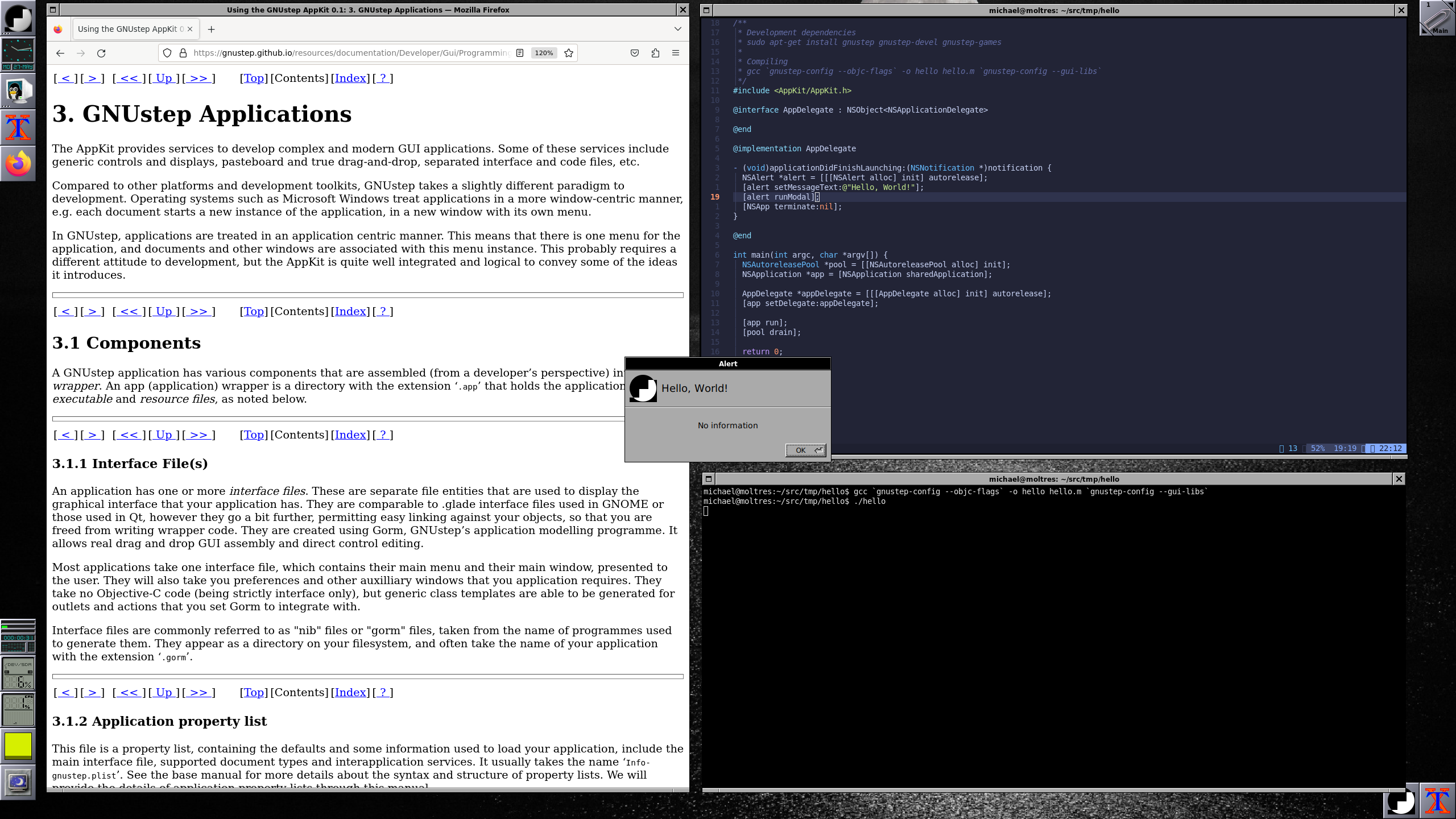
In today’s article we’ll setup a local environment for writing GNUstep programs, and we’ll also write and compile a simple “Hello, world” application to make sure everything is setup.
Brief History
GNUstep is an open-source implementation of the OpenStep specification, which originated from NeXT, a company founded by Steve Jobs after he left Apple in 1985. NeXT developed the NeXTSTEP operating system, which introduced an advanced object-oriented framework for software development. In 1993, NeXT partnered with Sun Microsystems to create the OpenStep standard, which aimed to make NeXT’s frameworks available on other platforms.
When Apple acquired NeXT in 1996, the technology from NeXTSTEP and OpenStep formed the foundation of Apple’s new operating system, Mac OS X. Apple’s Cocoa framework, a core part of macOS, is directly derived from OpenStep. GNUstep, initiated in the early 1990s, aims to provide a free and portable version of the OpenStep API, allowing developers to create cross-platform applications with a foundation rooted in the same principles that underpin macOS development.
So, this still leaves us with GNUstep to get up and running.
Developer environment
First up, we need to install all of the dependencies in our developer environment. I’m using Debian so all of my package management will be specific to that distribution. All of these packages will be available on all distributions though.
First of all, we include AppKit/AppKit.h so that we get access to the programming API. We then define our own AppDelegate so we capture the applicationDidFinishLaunching slot:
Now that we have our code written into hello.m, we can compile and link. There are some compile and link time libraries required to get this running. For this, we’ll use gnustep-config to do all of the heavy lifting for us.