One of the most important elements of any 3D application is its camera. A camera allows you to move around in your world and orient your view. In today’s post, I’ll put together a code walk through that will take you through a simple camera implementation.
The Concept
There are two major components of any camera. They are position and orientation. Position is fairly easy to grasp, it’s just where the camera is and is identified using a normal 3-space vector.
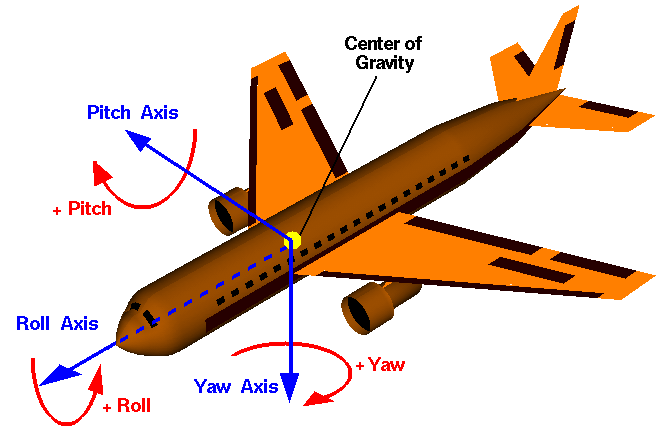
The more difficult of the two concepts is orientation. The best description for this that I’ve found is on the Flight Dynamics page on wikipedia. The following image has been taken from that article and it outlines the plains that orientation can occur. Of course, the image’s subject is an aircraft but the same concepts apply to a camera’s orientation:
The pitch describes the orientation around the x-axis, the yaw describes the orientation around the y-axis and the roll describes the orientation around the z-axis.
With all of this information on board, the requirements of our camera should become a little clearer. We need to keep track of the following about the camera:
Position
Up orientation (yaw axis)
Right direction (pitch axis)
Forward (or view) direction (roll axis)
We’ll also keep track of how far we’ve gone around the yaw, pitch and roll axis.
Some Maths (and code)
There’s a handful of really useful equations that are going to help us out here. With all of the information that we’ll be managing and how tightly related each axis is considering they’re all relating to the same object - you can see how interactive it can be just by modifying one attribute.
voidcamera::pitch(constfloatangle){// keep track of how far we've gone around the axisthis->rotatedX+=angle;// calculate the new forward vectorthis->viewDir=glm::normalize(this->viewDir*cosf(angle*PION180)+this->upVector*sinf(angle*PION180));// calculate the new up vectorthis->upVector=glm::cross(this->viewDir,this->rightVector);// invert so that positive goes downthis->upVector*=-1;}
voidcamera::yaw(constfloatangle){// keep track of how far we've gone around this axisthis->rotatedY+=angle;// re-calculate the new forward vectorthis->viewDir=glm::normalize(this->viewDir*cosf(angle*PION180)-this->rightVector*sinf(angle*PION180));// re-calculate the new right vectorthis->rightVector=glm::cross(this->viewDir,this->upVector);}
voidcamera::roll(constfloatangle){// keep track of how far we've gone around this axisthis->rotatedZ+=angle;// re-calculate the forward vectorthis->rightVector=glm::normalize(this->rightVector*cosf(angle*PION180)+this->upVector*sinf(angle*PION180));// re-calculate the up vectorthis->upVector=glm::cross(this->viewDir,this->rightVector);// invert the up vector so positive points downthis->upVector*=-1;}
Ok, so that’s it for orientation. Reading through the equations above, you can see that the calculation of the forward vector comes out of some standard rotations. The x operator that I’ve used above denotes vector cross product.
Now that we’re keeping track of our current viewing direction, up direction and right direction; performing camera movements is really easy.
I’ve called these advance (move along the forward plane), ascend (move along the up plane) and strafe (move along the right plane).
// z movementvoidcamera::advance(constfloatdistance){this->position+=(this->viewDir*-distance);}// y movementvoidcamera::ascend(constfloatdistance){this->position+=(this->upVector*distance);}// x movementvoidcamera::strafe(constfloatdistance){this->position+=(this->rightVector*distance);}
All we are doing here is just moving along those planes that have been defined for us via orientation. Movement is simple.
Integrating
All of this code/math is great up until we need to apply it in our environments. Most of the work that I do centralises around OpenGL, so I’ve got a very handy utility function (from GLU) that I use called gluLookAt. Plugging these values in is rather simple:
voidcamera::place(void){glm::vec3viewPoint=this->position+this->viewDir;// setup opengl with gluLookAtgluLookAt(position[0],position[1],position[2],viewPoint[0],viewPoint[1],viewPoint[2],upVector[0],upVector[1],upVector[2]);}
We calculate our viewpoint as (position - forwardVector) and really just plug the literal values into this function. There is a lot of information on the gluLookAt documentation page that you can use if OpenGL isn’t your flavor to simulate what it does.
GLUT is the OpenGL Utility Toolkit which is a standard set of APIs that you should be able to use on any platform to write OpenGL programs. It takes care of the boilerplate code that your applications would need to integrate with the host windowing system. More can be found about GLUT on its website.
Today’s post, I’ll focus on getting your Linux environment up to speed to start writing programs with this framework.
Installation
In order to write programs using this library, you’ll need to install the development library. Using your favorite package manager, you’ll need to install freeglut.
$ sudo apt-get install freeglut3-dev
After that’s finished, it’s time to write a test application to make sure everything went to plan.
A Simple Example
The following program will just open a window and continually clear the window.
#include<GL/glut.h>voidresize(intwidth,intheight){// avoid div-by-zeroif(height==0){height=1;}// calculate the aspect ratiofloatratio=width*1.0/height;// put opengl into projection matrix modeglMatrixMode(GL_PROJECTION);// reset the matrixglLoadIdentity();// set the viewportglViewport(0,0,width,height);// set the perspectivegluPerspective(45.0f,ratio,0.1f,100.0f);// put opengl back into modelview modeglMatrixMode(GL_MODELVIEW);}voidrender(void){// just clear the buffers for nowglClear(GL_COLOR_BUFFER_BIT|GL_DEPTH_BUFFER_BIT);// flip the buffersglutSwapBuffers();}intmain(intargc,char*argv[]){// initialize glutglutInit(&argc,argv);// setup a depth buffer, double buffer and rgba modeglutInitDisplayMode(GLUT_DEPTH|GLUT_DOUBLE|GLUT_RGBA);// set the windows initial position and sizeglutInitWindowPosition(50,50);glutInitWindowSize(320,240);// create the windowglutCreateWindow("Test Glut Program");// register the callbacks to glutglutDisplayFunc(render);glutReshapeFunc(resize);glutIdleFunc(render);// run the programglutMainLoop();return0;}
Putting this code into “test.c”, we built it into a program with the following command:
$ gcc test.c -lGL-lGLU-lglut-otest
That’s it! Run “test” at the command prompt and if everything has gone to plan, you’ve installed freeglut correctly!
In a previous article I’d put together a walk through on how to get your development environment ready to write some OpenCL code. This article by itself isn’t of much use unless you can write some code already. Today’s post will be a walk through on writing your first OpenCL program. This example, much like a lot of the other entry-level OpenCL development tutorials will focus on performing addition between two lists of floating point numbers.
Lots to learn
Unfortunately, OpenCL is a topic that brings a very steep learning curve. In order to understand even the most simple of programs you need to read a fair bit of code and hopefully be aware of what it’s doing. Before we dive into any implementation, I’ll take you on a brief tour of terms, types and definitions that will help you to understanding the code as it’s presented.
A cl_platform_id is obtained using clGetPlatformIDs. A platform in OpenCL refers to the host execution environment and any attached devices. Platforms are what allow OpenCL to share resources and execute programs.
A cl_device_id is obtained using clGetDeviceIDs. It’s how your program will refer to the devices that your code will run on. A device is how OpenCL refers to “something” that will execute code (CPU, GPU, etc).
A cl_context is obtained using clCreateContext. A context is established across OpenCL devices. It’s what OpenCL will use to manage command-queues, memory, program and kernel objects. It provides the ability to execute a kernel across many devices.
A cl_program is created from actual (string) source-code at runtime using clCreateProgramWithSource. They’re created in conjunction with your context so that program creation is aware of where it’ll be expected to run. After the cl_program reference is successfully established, the host program would typically call clBuildProgram to take the program from its source code (string) state into an executable (binary) state.
A cl_command_queue is established using clCreateCommandQueue. A command queue is how work is scheduled to a device for execution.
A cl_kernel is created using clCreateKernel. A kernel is a function contained within a compiled cl_program object. It’s identified within the source code with a __kernel qualifier. You set the argument list for a cl_kernel object using clSetKernelArg. To glue it all together, you use clEnqueueNDRangeKernel or clEnqueueTask to enqueue a task on the command queue to execute a kernel.
A side note here is that you can use clEnqueueNativeKernel to execute native C/C++ code that isn’t compiled by OpenCL.
At least if you can identify some form of meaning when you come across these type names, you won’t be totally in the dark. Next up, we’ll create a host program and OpenCL routine - compile, build and run!
The Host
The host application is responsible for engaging with the OpenCL api to setup all of the objects described above. It’s also responsible for locating the OpenCL source code and making it available for compilation at run time. In this first snippet of code, we use the OpenCL api to establish the management platform and devices that are available to execute our code. Majority of the OpenCL api standardises itself around returning error codes from all of the functions.
cl_platform_idplatform;cl_device_iddevice;interr;/* find any available platform */err=clGetPlatformIDs(1,&platform,NULL);/* determine if we failed */if(err<0){perror("Unable to identify a platform");exit(1);}/* try to acquire the GPU device */err=clGetDeviceIDs(platform,CL_DEVICE_TYPE_GPU,1,&device,NULL);/* if no GPU was found, fail-back to the CPU */if(err==CL_DEVICE_NOT_FOUND){err=clGetDeviceIDs(platform,CL_DEVICE_TYPE_CPU,1,&device,NULL);}/* check that we did acquire a device */if(err<0){perror("Unable to acquire any devices");exit(1);}
At this point, we have “platform” which will (hopefully) contain a platform ID identifying our management platform and “device” should either refer to the GPU or CPU (failing to find a GPU). The next step is to create a context and your OpenCL program from source.
/* we'll get to this soon. for the time being, imagine that your
OpenCL source code is located by the following variable */char*program_source=". . .";size_tprogram_size=strlen(program_source);cl_contextcontext;cl_programprogram;/* try to establish a context with the device(s) that we've found */context=clCreateContext(NULL,1,&device,NULL,NULL,&err);/* check that context creation was successful */if(err<0){perror("Unable to create a context");exit(1);}/* using the context, create the OpenCL program from source */program=clCreateProgramWithSource(context,1,(constchar**)&program_source,&program_size,&err);/* chech that we could create the program */if(err<0){perror("Unable to create the program");exit(1);}
We’ve done just that here, but the program isn’t quite yet ready for execution. Before we can start using this, we need to build the program. The build process is very much a compilation & linking process that involves its own set of log message outputs, etc. You can make this part of your program as elaborate as you’d like. Here’s an example compilation process.
size_tlog_size;char*program_log;/* build the program */err=clBuildProgram(program,0,NULL,NULL,NULL,NULL);/* determine if the build failed */if(err<0){/* the build has failed here, so we'll now ask OpenCL for the build
information, so that we can display the errors back to the user *//* pull back the size of the log */clGetProgramBuildInfo(program,device,CL_PROGRAM_BUILD_LOG,0,NULL,&log_size);/* allocate a buffer and draw the log into a string */program_log=(char*)malloc(log_size+1);program_log[log_size]='\0';/* pull back the actual log text */clGetProgramBuildInfo(program,device,CL_PROGRAM_BUILD_LOG,log_size+1,program_log,NULL);/* send the log out to the console */printf("%s\n",program_log);free(program_log);exit(1);}
We’ve got a platform, device, context and program that’s been built. We now need to shift contexts from the host program to the actual OpenCL code that we’ll execute for the purposes of this example. We need to understand what the inputs, outputs, used resources, etc. of the OpenCL code is before we can continue to write the rest of our host.
The OpenCL Code
The main purpose of OpenCL code is really to operate arithmetically on arrays (or strings) of data. The example that I’m suggesting for the purposes of this article takes in two source arrays and produces another array which are the sum of each index. i.e.
c[0] = a[0] + b[0]
c[1] = a[1] + b[1]
. . .
. . .
As above, the source arrays are a and b. The result array (holding the sum of each source array at each index) is c. Here’s the (rather simple) OpenCL code to achieve this.
__kernelvoidadd_numbers(__globalconstint*a,__globalconstint*b,__globalint*c){// get the array index we're going to work onsize_tidx=get_global_id(0);// sum the valuesc[idx]=a[idx]+b[idx];}
That’s all there is to it. Things to note are, any function that is to be called in the OpenCL context is called a “kernel”. Kernel’s must be decorated with the __kernel modifier. In this example, the parameters that are passed in are decorated with the __global modifier. This tells OpenCL that these are objects allocated from the global memory pool. You can read up more about these modifiers here. The final thing to note is the use of get_global_id. It’s what gives us the particular index to process in our array here. The parameter that’s supplies allows you to work with 1, 2 or 3 dimensional arrays. Anything over this, the arrays need to be broken down to use a smaller dimension count.
Back to the Host
Back in context of the host, we’ll create the command queue and kernel objects. The command queue allows us to send commands to OpenCL like reading & writing to buffers or executing kernel code. The following code shows the creation of the command queue and kernel.
cl_command_queuequeue;cl_kernelkernel;/* create the command queue */queue=clCreateCommandQueue(context,device,0,&err);/* check that we create the queue */if(err<0){perror("Unable to create a command queue");exit(1);}/* create the kernel */kernel=clCreateKernel(program,"add_numbers",&err);/* check that we created the kernel */if(err<0){perror("Unable to create kernel");exit(1);}
Notice that we mentioned the kernel by name here. A kernel object refers to the function! Now that we have a function to execute (or kernel) we now need to be able to pass data to the function. We also need to be able to read the result once processing has finished. Our first job is allocating buffers that OpenCL will be aware of to handle these arrays.
/* here are our source data arrays. "ARRAY_SIZE" is defined elsewhere to
give these arrays common bounds */inta_data[ARRAY_SIZE],b_data[ARRAY_SIZE],c_data[ARRAY_SIZE];/* these are the handles that OpenCL will refer to these memory chunks */cl_mema_buffer,b_buffer,c_buffer;/* initialize a_data & b_data to integers that we want to add */for(i=0;i<ARRAY_SIZE;i++){a_data[i]=random()%1000;b_data[i]=random()%1000;}/* create the memory buffer objects */a_buffer=clCreateBuffer(context,CL_MEM_READ_ONLY,ARRAY_SIZE*sizeof(int),NULL,&err);b_buffer=clCreateBuffer(context,CL_MEM_READ_ONLY,ARRAY_SIZE*sizeof(int),NULL,&err);c_buffer=clCreateBuffer(context,CL_MEM_READ_WRITE,ARRAY_SIZE*sizeof(int),NULL,&err);
In the above snippet, we’ve defined the source arrays and we’ve also created buffers that will hold the information (for use in our OpenCL code). Now all we need to do is to feed the source arrays into the buffers and supply all of the buffers as arguments to our kernel.
/* fill the source array buffers */err=clEnqueueWriteBuffer(queue,a_buffer,CL_TRUE,0,ARRAY_SIZE*sizeof(int),a_data,0,NULL,NULL);err=clEnqueueWriteBuffer(queue,b_buffer,CL_TRUE,0,ARRAY_SIZE*sizeof(int),b_data,0,NULL,NULL);/* supply these arguments to the kernel */err=clSetKernelArg(kernel,0,sizeof(cl_mem),&a_buffer);err=clSetKernelArg(kernel,1,sizeof(cl_mem),&b_buffer);err=clSetKernelArg(kernel,2,sizeof(cl_mem),&c_buffer);
Now we invoke OpenCL to do the work. In doing this, we need to supply the invocation with a global size and local size. Global size is used to specify the total number of work items being processed. In our case, this is ARRAY_SIZE. Local size is used as the number of work items in each local group. Local size needs to be a divisor of global size. For simplicity, I’ve set these both to ARRAY_SIZE.
intglobal_size=ARRAY_SIZE,local_size=ARRAY_SIZE;/* send the work request to the queue */err=clEnqueueNDRangeKernel(queue,kernel,1,NULL,&global_size,&local_size,0,NULL,NULL);/* check that we could queue the work */if(err<0){perror("Unable to queue work");exit(1);}/* wait for the work to complete */clFinish(queue);
After all of the work is completed, we really want to take a look at the result. We’ll send another request to the command queue to read that result array back into local storage. From there, we’ll be able to print the results to screen.
/* read out the result array */err=clEnqueueReadBuffer(queue,c_buffer,CL_TRUE,0ARRAY_SIZE*sizeof(int),c_data,0,NULL,NULL);/* check that the read was ok */if(err<0){perror("Unable to read result array");exit(1);}/* print out the result */for(i=0;i<ARRAY_SIZE;i++){printf("%d + %d = %d\n",a_data[i],b_data[i],c_data[i]);}
Fantastic. Everything’s on screen now, we can see the results. All we’ll do from here is clean up our mess and get out.
OpenCL (or Open Computing Language) is a framework that allows you to write code across different connected devices to your computer. Code that you write can execute on CPUs, GPUs, DPSs amongst other pieces of hardware. The framework itself is a standard that puts the focus on running your code across these devices but also emphasises parallel computing.
Today’s post will just be on getting your development environment setup on Debian Wheezy to start writing some code.
Installation
The installation process is pretty straight forward, but there are some choices in libraries. The major vendors (Intel, NVIDIA and AMD) all have development libraries that are installable from Debian’s package repository. There’s plenty of banter on the internet as to who’s is better for what purpose.
First off, we need to install the header files we’ll use to create OpenCL programs.
$ sudo apt-get install opencl-headers
This has now put all of the development headers in place for you to compile some code.
$ ls -al /usr/include/CL
total 1060
drwxr-xr-x  2 root root   4096 Nov 25 22:51 .
drwxr-xr-x 56 root root   4096 Nov 25 22:51 ..
-rw-r--r--  1 root root   4859 Nov 15  2011 cl_d3d10.h
-rw-r--r--  1 root root   4853 Apr 18  2012 cl_d3d11.h
-rw-r--r--  1 root root   5157 Apr 18  2012 cl_dx9_media_sharing.h
-rw-r--r--  1 root root   9951 Nov 15  2011 cl_ext.h
-rw-r--r--  1 root root   2630 Nov 17  2011 cl_gl_ext.h
-rw-r--r--  1 root root   7429 Nov 15  2011 cl_gl.h
-rw-r--r--  1 root root  62888 Nov 17  2011 cl.h
-rw-r--r--  1 root root 915453 Feb  4  2012 cl.hpp
-rw-r--r--  1 root root  38164 Nov 17  2011 cl_platform.h
-rw-r--r--  1 root root   1754 Nov 15  2011 opencl.h
Secondly, we need to make a choice in what library we’ll use:
The amd-opencl-dev package will install AMD’s implementation, which you can read up on here. NVIDIA’s package is installable through the nvidia-opencl-dev package which you can read up on here. Finally, Intel’s implementation is available through the beignet-dev package and you can read up on their implementation here.
I went with AMD’s.
$ sudo apt-get install amd-opencl-dev
From here, it’s time to write some code. I’ll have some more blog posts on the way which will be walk-throughs for your first applications.
In my previous post, we went through the basics of rasterising polygons on screen by use of horizontal lines. To sum up, we interpolated values along each edge of the polygon, collecting minimum and maximums for each y-axis instance.
Today, we’re going to define a colour value for each point on the polygon and interpolate the colours along each edge. This is the technique employed to draw polygons that are Gouraud shaded.
The Code
The structure of this is very similar to drawing a single colour block polygon. For a solid colour polygon, we interpolated the x values over the length of the y values. We’ll now employ this same interpolation technique over the red, green, blue and alpha channels of each colour defined for each polygon point. Here’s the scanline function.
varscanline_g=function(p1,p2,miny,edges){// if the y values aren't y1 < y2, flip them// this will also flip the colour componentsif(p2.y<p1.y){varp=p1;p1=p2;p2=p;}// initialize our counters for the x-axis, r, g, b and a colour componentsvarx=p1.x;varr=p1.r,g=p1.g,b=p1.b,a=p1.a;// calculate the deltas that we'll use to interpolate along the length of// the y-axis here (y2 - y1)varyLen=p2.y-p1.y;vardx=(p2.x-p1.x)/yLen;vardr=(p2.r-p1.r)/yLen;vardg=(p2.g-p1.g)/yLen;vardb=(p2.b-p1.b)/yLen;varda=(p2.a-p1.a)/yLen;// find our starting array indexvarofs=p1.y-miny;// enumerate each point on the y axisfor(vary=p1.y;y<=p2.y;y++){// test if we have a new minimum, and if so save itif(edges[ofs].min.x>x){edges[ofs].min.x=Math.floor(x);edges[ofs].min.r=Math.floor(r);edges[ofs].min.g=Math.floor(g);edges[ofs].min.b=Math.floor(b);edges[ofs].min.a=Math.floor(a);}// test if we have a new maximum, and if so save itif(edges[ofs].max.x<x){edges[ofs].max.x=Math.floor(x);edges[ofs].max.r=Math.floor(r);edges[ofs].max.g=Math.floor(g);edges[ofs].max.b=Math.floor(b);edges[ofs].max.a=Math.floor(a);}// move our interpolators along their respective pathsx+=dx;r+=dr;g+=dg;b+=db;a+=da;// move to the next array offsetofs++;}};
An immediate code restructure difference here from the first tutorial, is I’m now passing an actual point object through as opposed to each component of each point being a function parameter. This is just to clean up the interface of these functions. We’re creating differentials not only for x now but also the r, g, b and a components. These will form the start and ending colours for each horizontal line that we’ll draw. We still have extra interpolation to do once we’re in the horizontal line draw function as well. Here it is.
varhline_g=function(x1,x2,y,w,c1,c2,buffer){// calculate the starting offset to draw atvarofs=(x1+y*w)*4;// calculate the length of the linevarlineLength=x2-x1;// calculate the deltas for the red, green, blue and alpha channelsvardr=(c2.r-c1.r)/lineLength;vardg=(c2.g-c1.g)/lineLength;vardb=(c2.b-c1.b)/lineLength;varda=(c2.a-c1.a)/lineLength;// initialize our countersvarr=c1.r,g=c1.g,b=c1.b,a=c1.a;// interpolate every position on the x axisfor(varx=x1;x<=x2;x++){// draw this coloured pixelbuffer[ofs]=Math.floor(r);buffer[ofs+1]=Math.floor(g);buffer[ofs+2]=Math.floor(b);buffer[ofs+3]=Math.floor(g);// move the interpolators onr+=dr;g+=dg;b+=db;a+=da;// move to the next pixrlofs+=4;}};
Again, more interpolation of colour components. This is what will give us a smooth shading effect over the polygon. Finally, the actual polygon function is a piece of cake. It just gets a little more complex as we have to send in colours for each point defined.
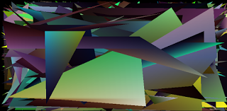
varpolygon_g=function(p1,p2,p3,p4,w,buffer){// work out the minimum and maximum y values for the polygonvarminy=p1.y,maxy=p1.y;if(p2.y>maxy)maxy=p2.y;if(p2.y<miny)miny=p2.y;if(p3.y>maxy)maxy=p3.y;if(p3.y<miny)miny=p3.y;if(p4.y>maxy)maxy=p4.y;if(p4.y<miny)miny=p4.y;varh=maxy-miny;varedges=newArray();// create the edge storage so we can keep track of minimum x, maximum x// and corresponding r, g, b, a componentsfor(vari=0;i<=h;i++){edges.push({min:{x:1000000,r:0,g:0,b:0,a:0},max:{x:-1000000,r:0,g:0,b:0,a:0}});}// perform the line scans on each polygon egdescanline_g(p1,p2,miny,edges);scanline_g(p2,p3,miny,edges);scanline_g(p3,p4,miny,edges);scanline_g(p4,p1,miny,edges);// enumerate over all of the edge itemsfor(vari=0;i<edges.length;i++){// get the start and finish colourc1={r:edges[i].min.r,g:edges[i].min.g,b:edges[i].min.b,a:edges[i].min.a};c2={r:edges[i].max.r,g:edges[i].max.g,b:edges[i].max.b,a:edges[i].max.a};// draw the linehline_g(edges[i].min.x,edges[i].max.x,i+miny,w,c1,c2,buffer);}};
Aside from the interface changing (just to clean it up a bit) and managing r, g, b and a components - this hasn’t really changed from the block colour version. If you setup this polygon draw in a render loop, you should end up with something like this: