Performance Monitoring a Linux Environment
11 Jul 2013This post is just a list of links I’ve collected for looking at a Linux system’s performance.
This post is just a list of links I’ve collected for looking at a Linux system’s performance.
This post is just a list of bookmarks I’ll keep to refer to for MongoDB performance analysis.
One of the first things that I reach for when writing an application that will be used outside the context of my development sandbox is a configuration library. Not having statically compiled values for variables is quite a valuable position to be in once your application has been deployed. Today’s post will take you from 0 to up and running with a package called ConfigFile that is specifically designed to serve your applications with configuration data. Most of the content in this post is lifted directly from the documentation, so you’ll be better off reading through those to gain a deeper understanding of the library. This post is more of a short-cut to get up and running.
If you’ve had much experience with administering windows back in the day when INI files ruled the earth, you’ll be right at home with ConfigFile. For those of you who have never seen it before, it’s really easy and you can read up on it here. Files are broken into sections which contain a list of key/value pairs - done!
For today’s example, the configuration file will look as follows:
[Location]
path=/tmp
filename=blah
We’ll end up with two keys, path and filename that have corresponding values in the Location section.
The thing I like most about the part of the application is that we can make a nice record based data structure in Haskell that will marry up to how our configuration file looks. The simple file that we’ve defined above, would look like this:
data ConfigInfo = ConfigInfo { path :: String
                             , fileName :: String
                             }
Once we fill one of these up, you can see that it’ll be pretty natural to access these details.
Finally - we need to read the values out of the config file and get them into our structure. The following block of code will do that for us.
readConfig :: String -> IO ConfigInfo
readConfig f = do
   rv <- runErrorT $ do

      -- open the configuration file
      cp <- join $ liftIO $ readfile emptyCP f
      let x = cp

      -- read out the attributes
      pv <- get x "Location" "path"
      fv <- get x "Location" "filename"

      -- build the config value
      return (ConfigInfo { path = pv
                         , fileName = fv
                         })

   -- in the instance that configuration reading failed we'll
   -- fail the application here, otherwise send out the config
   -- value that we've built
   either (\x -> error (snd x)) (\x -> return x) rv
There’s a few interesting points in here to note. The Error Monad is being used here to keep track of any failures during the config read process. runErrorT kicks this off for us. We then use readfile to open the config file with a sane parser that knows how to speak INI. Pulling the actual strings from the config is done by using get. From here, it’s just wrapping the values up ready to send out. The final call is to either. Leaving the Error Monad, we’re given an Either (left being the error, right being the value). I’ve used either here so I can provide an implementation for either scenario. If an error occurs (the first lambda) then I just toast-out of the application. If we get a config value back (the second lambda), that’s what gets returned.
That’s all there is to that. Remember, you won’t escape from the IO Monad which is why the read function’s return type has IO. When you want to use these values, it’ll need to be within do constructs:
main :: IO ()
main = do
   config <- readConfig "test.cfg"
   putStrLn $ "The path value is: " ++ (path config)
   putStrLn $ "The filename value is: " ++ (fileName config)
Cheers.
Working in a Linux environment for more and more of the day, it pays to know your tools really well. One tool that I use frequently to understand what a machine is doing is the top command. Today’s post will take you through all of the figures on this report to help you understand what each means.
The top command is a very common tool used to “display Linux tasks” as the man page so helpfully tells us. Issuing this command at the shell will present the user with a few rows of figures followed by a list of all running processes on the system. Here is an extract of the report (just the upper lines that this post will focus on).
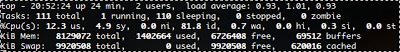
You can see from the excerpt above that quite a lot of information is packed into this part of the report. To breakdown this report, I’ll just got through it line by line.
top - 20:52:24 up 24 min, 2 users, load average: 0.93, 1.01, 0.93The first line tells us the following:
The system load average is an interesting one. A general rule of thumb is to investigate if you’re seeing averages above 0.7. An average of 1.0 suggests that just enough work is getting processed by the machine, but is leaving you no headroom to move. Seeing a load of 5 and above is panic-time, systems stalling, trouble. For more information about these load values, take a look at Understanding Linux CPU Load - when should you be worried?
Tasks: 111 total, 1 running, 110 sleeping, 0 stopped, 0 zombieThe second line tells us the following:
%Cpu(s): 12.3 us, 4.9 sy, 0.0 ni, 81.8 id, 0.7 wa, 0.0 hi, 0.3 si, 0.0 stThe third line gives you a point in time view of how busy the CPU is and where its cycles are being used. It tells us the percentage of CPU being used for:
KiB Mem:   8129072 total,  1402664 used,  6726408 free,    69512 buffers
KiB Swap:  9920508 total,        0 used,  9920508 free,   620016 cached
The fourth and fifth lines deal with memory and swap utilisation. It tells us the following:
That’s it for the summary of the machine’s activity. These are all the aggregate values which will give you an “at a glance” feel for how the machine is going. The next part of this post will be all about reading specific information from the process report. Here’s an excerpt of the report.

To interrogate a single process, you can use the details within the process report. It will list out all of the processes currently managed by your system. The report columns as you look at it will provide the following information:
That’s it for the “top” command in Linux. Remember, always read the man pages for commands that you want to learn more about!
Getting a wider array of fonts into your website is a pretty simple task these days. There’s quite a selection of fonts that you can use offered on the web. Just take a look at Google’s repository to see what I’m talking about.
Once you’ve selected the font that’s right for your application, you can import it to pages using the following directive:
@import url(http://fonts.googleapis.com/css?family=Droid+Sans:400,700);… and then finally use it in your css directives.
font-family: "Droid Sans", arial, verdana, sans-serif;Easy.