D-Bus

Introduction

D-Bus (Desktop Bus) is an inter-process communication (IPC) system used on Linux and other Unix-like systems. It allows different programs — even running as different users — to send messages and signals to each other without needing to know each other’s implementation details.

Main ideas

• Message bus: A daemon (dbus-daemon) runs in the background and acts as a router for messages between applications.
• Two main buses:
  • System bus – for communication between system services and user programs (e.g., NetworkManager, systemd, BlueZ).
  • Session bus – for communication between applications in a user’s desktop session (e.g., a file manager talking to a thumbnailer).
• Communication model:
  • Method calls – like function calls between processes.
  • Signals – broadcast events (e.g., “Wi-Fi disconnected”).
  • Properties – read/write state values.
• Naming:
  • Bus names – unique or well-known IDs for services (e.g., org.freedesktop.NetworkManager).
  • Object paths – hierarchical paths (e.g., /org/freedesktop/NetworkManager).
  • Interfaces – namespaces for methods/signals (e.g., org.freedesktop.NetworkManager.Device).

Here’s a visual representation of the architecture:

User applications call methods or raise signals to a Session Bus inside the D-Bus Daemon. In turn, these messages are routed to System Services, with responses sent back to the applications via the bus.

D-Bus removes the need for each program to implement its own custom IPC protocol. It’s widely supported by desktop environments, system services, and embedded Linux stacks.

In this article, we’ll walk through some basic D-Bus usage, building up to a few practical use cases.

busctl

busctl lets you interact with D-Bus from the terminal. According to the man page:

busctl may be used to introspect and monitor the D-Bus bus.

We can start by listing all connected peers:

busctl list

This shows a list of service names for software and services currently on your system’s bus.

Devices

If you have NetworkManager running, you’ll see org.freedesktop.NetworkManager in the list.
You can query all available devices with:

busctl call org.freedesktop.NetworkManager /org/freedesktop/NetworkManager \
  org.freedesktop.NetworkManager GetDevices

Example output:

ao 6 "/org/freedesktop/NetworkManager/Devices/1" "/org/freedesktop/NetworkManager/Devices/2" "/org/freedesktop/NetworkManager/Devices/3" "/org/freedesktop/NetworkManager/Devices/4" "/org/freedesktop/NetworkManager/Devices/5" "/org/freedesktop/NetworkManager/Devices/6"

Those object paths aren’t very descriptive, so you can query one for its interface name:

busctl get-property org.freedesktop.NetworkManager \
  /org/freedesktop/NetworkManager/Devices/1 \
  org.freedesktop.NetworkManager.Device Interface

On my system:

s "lo"

The leading s tells us this is a string — here, the loopback adapter.

Introspect

You can list all properties, methods, and signals for a given object with:

busctl introspect org.freedesktop.NetworkManager \
  /org/freedesktop/NetworkManager/Devices/1

Or without the pager:

busctl --verbose --no-pager introspect org.freedesktop.NetworkManager \
  /org/freedesktop/NetworkManager/Devices/1

Desktop Notifications

Now that we can query D-Bus, we can also send messages.
For example, you could end a shell script with a visual notification on your desktop:

gdbus call --session \
  --dest org.freedesktop.Notifications \
  --object-path /org/freedesktop/Notifications \
  --method org.freedesktop.Notifications.Notify \
  "my-app" 0 "" "Build finished" "All tests passed" \
  '[]' '{"urgency": <byte 1>}' 5000

Tip: gdbus is part of the glib2 or glib2-tools package on many distributions.

This performs a method call on a D-Bus object.

• --dest — The bus name (service) to talk to.
• --object-path — The specific object inside that service.
• --method — The method we want to invoke.

This method’s signature is s u s s s as a{sv} i, meaning:

Monitoring

D-Bus also lets you watch messages as they pass through.
To monitor all system bus messages (root may be required):

busctl monitor --system

To filter for a specific destination:

busctl monitor org.freedesktop.NetworkManager

These commands stream events to your console in real time.

Conclusion

D-Bus is a quiet but powerful layer in modern Linux desktops and servers. Whether you’re inspecting running services, wiring up automation, or building new desktop features, learning to speak D-Bus gives you a direct line into the heart of the system. Once you’ve mastered a few core commands, the rest is just exploring available services and imagining what you can automate next.

Move Semantics in C++

TL;DR: std::move doesn’t move anything by itself. It’s a cast that permits moving. Real moves happen in your type’s move constructor/assignment. Use them to trade deep copies for cheap pointer swaps and to unlock container performance—provided you mark them noexcept.

The motivating example

We’ll anchor everything on a tiny heap-owning type. It’s intentionally “unsafe” (raw new[]/delete[]) so the ownership transfer is easy to see in logs.

#include <iostream>
#include <utility> // for std::move

struct my_object {
    int* data;
    size_t size;

    // Constructor
    my_object(size_t n) : data(new int[n]), size(n) {
        std::cout << "Constructed (" << this << ") size=" << size 
                  << " data=" << data << "\n";
    }

    // Copy constructor
    my_object(const my_object& other) 
        : data(new int[other.size]), size(other.size) {
        std::copy(other.data, other.data + size, data);
        std::cout << "Copied from (" << &other << ") to (" << this << ")"
                  << " data=" << data << "\n";
    }

    // Move constructor
    my_object(my_object&& other) noexcept 
        : data(other.data), size(other.size) {
        other.data = nullptr;
        other.size = 0;
        std::cout << "Moved from (" << &other << ") to (" << this << ")"
                  << " data=" << data << "\n";
    }

    // Destructor
    ~my_object() {
        std::cout << "Destroying (" << this << ") data=" << data << "\n";
        delete[] data;
    }
};

int main() {
    std::cout << "--- Create obj1 ---\n";
    my_object obj1(5);

    std::cout << "\n--- Copy obj1 into obj2 ---\n";
    my_object obj2 = obj1; // Calls copy constructor

    std::cout << "\n--- Move obj1 into obj3 ---\n";
    my_object obj3 = std::move(obj1); // Calls move constructor

    std::cout << "\n--- End of main ---\n";
}

When you run this you’ll see:

• One deep allocation
• One deep copy (new buffer), and
• One move (no allocation; just pointer steal).

The destructor logs reveal that ownership was transferred and that the moved-from object was neutered.

Try it: clang++ -std=c++20 -O0 -g move_demo.cpp && ./a.out

Having a brief look at the output (from my machine, at least):

--- Create obj1 ---
Constructed (0x7ffd8c960858) size=5 data=0x5616824336c0

--- Copy obj1 into obj2 ---
Copied from (0x7ffd8c960858) to (0x7ffd8c960848) data=0x5616824336e0

--- Move obj1 into obj3 ---
Moved from (0x7ffd8c960858) to (0x7ffd8c960838) data=0x5616824336c0

--- End of main ---
Destroying (0x7ffd8c960838) data=0x5616824336c0
Destroying (0x7ffd8c960848) data=0x5616824336e0
Destroying (0x7ffd8c960858) data=0

• Constructed: obj1 allocates a buffer at 0x5616824336c0.
• Copied: obj2 gets its own buffer (0x5616824336e0) and the contents are duplicated from obj1. At this point, both obj1 and obj2 own separate allocations.
• Moved: obj3 simply takes ownership of obj1’s buffer (0x5616824336c0) without allocating. obj1’s data pointer is nulled out (data=0), leaving it valid but empty.
• Destruction order: obj3 frees obj1’s original buffer, obj2 frees its own copy, and finally obj1 frees nothing (because it’s been neutered by the move).

The contrasting addresses make it easy to see:

• Copies produce different data pointers.
• Moves result in pointer reuse.

What problem do move semantics solve?

Before C++11, passing/returning big objects often meant deep copies or awkward workarounds. Containers like std::vector<T> also had a problem: on reallocation they could only copy elements. If copying T was expensive or forbidden, performance cratered.

Move semantics (C++11) let a type say: “If you no longer need the source object, I can steal its resources instead of allocating/copying them.” This unlocks:

• Returning large objects by value efficiently.
• Growing containers without copying payloads.
• Expressing one-time ownership transfers cleanly.

Conclusion

In this small example we only wrote a move constructor, but real-world resource-owning classes often need both move and copy operations, plus move assignment. The full “rule of five” ensures your type behaves correctly in all situations — and marking moves noexcept can make a big difference in container performance.

Move semantics solves a big problem especially when your class encapsulates a lot of data. It’s an elegant solution that C++ provides you for performance, ownership, and safety.

Building a Modular Synth in Clojure

Introduction

I’ve always liked the idea that a programming language can feel like a musical instrument.
Last night, I decided to make that idea very literal.

The result is rack — a little Clojure module that models a modular synthesizer. It doesn’t aim to be a complete DAW or polished softsynth — this is more of an experiment: what if we could patch together oscillators and filters the way Eurorack folks do, but using s-expressions instead of patch cables?

As always, the code for this article is up in my Github account to help you follow along.

Why Clojure Feels Like a Good Fit

Clojure’s s-expressions are perfect for this kind of modeling.

A synth module is, in some sense, just a little bundle of state and behavior. In OOP we might wrap that up in a class; in Clojure, we can capture it as a simple map, plus a few functions that know how to work with it.

The parentheses give us a “patch cable” feel — data and functions connected in readable chains.

A 30-Second Synth Primer

Before we dive into code, a very quick crash course in some synth lingo:

• VCO (Voltage-Controlled Oscillator): Produces a periodic waveform — the basic sound source.
• LFO (Low-Frequency Oscillator): Like a VCO, but slower, used for modulation (wobble, vibrato, etc.).
• VCA (Voltage-Controlled Amplifier): Controls the amplitude of a signal, usually over time.

That’s enough to make the examples readable. We’re here for the Clojure, not the audio theory.

Setup Audio

The first thing we need to do is open an audio output line.

Java’s javax.sound.sampled API is low-level but accessible from Clojure with no extra dependencies.

Here’s the start of our code:

(def ^:const sample-rate 48000.0)
(def ^:const bits-per-sample 16)
(def ^:const channels 1)

Three constants — a 48 kHz sample rate (good quality, not too CPU-heavy), 16-bit samples, and mono output.

Starting the Audio Engine

(defn ^SourceDataLine open-line
  ([] (open-line sample-rate))
  ([sr]
   (let [fmt (AudioFormat. (float sr) bits-per-sample channels true false) ; signed, little endian
         ^SourceDataLine line (AudioSystem/getSourceDataLine fmt)]
     (.open line fmt 4096)  ;; important: use (fmt, bufferSize) overload
     (.start line)
     line)))

Line by line:

1. Function arity: With no arguments, open-line uses our default sample rate. With one argument, you can pass a custom rate.
2. AudioFormat.: Creates a format object with:
   • sr as a float
   • bits-per-sample bits per sample
   • channels (mono)
   • true for signed samples
   • false for little-endian byte order
3. AudioSystem/getSourceDataLine: Asks the JVM for a line that matches our format.
4. .open: Opens the line with a buffer size of 4096 bytes — small enough for low latency, large enough to avoid dropouts.
5. .start: Starts audio playback.
6. Returns the SourceDataLine object so we can write samples to it.

Finding available outputs

(defn list-mixers []
  (doseq [[i m] (map-indexed vector (AudioSystem/getMixerInfo))]
    (println i ":" (.getName m) "-" (.getDescription m))))

This helper prints out all available audio devices (“mixers”) so you can choose one if your machine has multiple outputs. In cases where you’re struggling to find the appropriate sound mixer, this function can help you diagnose these problems.

Starting, Stopping, and Writing Audio

Opening an audio line is one thing — actually feeding it samples in real time is another.
This is where we start talking about frames, buffers, and a little bit of number crunching.

Writing audio frames

(defn- write-frames! [^SourceDataLine line ^floats buf nframes]
  (let [^bytes out (byte-array (* 2 nframes))]
    (dotimes [i nframes]
      (let [s (int (Math/round (* 32767.0 (double (aget buf i)))))
            idx (* 2 i)]
        (aset-byte out idx       (unchecked-byte (bit-and s 0xFF)))
        (aset-byte out (inc idx) (unchecked-byte (bit-and (unsigned-bit-shift-right s 8) 0xFF)))))
    (.write line out 0 (alength out))))

Here’s what’s happening:

1. Input:
   • buf: A float array of audio samples, each in the range \([-1.0, 1.0]\).
   • nframes: How many samples we want to send.
2. Output:
   • out: A byte array holding the samples in 16-bit little-endian PCM format.

Scaling floats to integers

Most audio hardware expects integers, not floats. In 16-bit PCM, the range is \([-32768, 32767]\).

We scale a float \(x\) by \(32767.0\):

For example:

(close enough; the exact min value is special-cased in PCM)

Breaking into bytes

Because 16 bits = 2 bytes, we split the integer into:

• Low byte: \(s \,\&\, 0xFF\)
• High byte: \((s \gg 8) \,\&\, 0xFF\)

We store them in little-endian order — low byte first — so the audio hardware interprets them correctly.

Stopping audio cleanly

(defn stop-audio! []
  (when (:running? @engine)
    (swap! engine assoc :running? false)
    (when-let [t (:thread @engine)]
      (try (.join t 500) (catch Throwable _))))
  (when-let [^SourceDataLine line (:line @engine)]
    (try (.drain line) (.stop line) (.close line)
         (catch Throwable _)))
  (reset! engine {:running? false :thread nil :line nil})
  :ok)

Stopping audio isn’t just hitting a “pause” button:

• :running? tells the audio thread to exit its loop.
• .join waits briefly for that thread to finish.
• .drain ensures any remaining samples in the buffer are played before stopping.
• .stop and .close free the hardware resources.

Starting audio in real time

(defn start-audio!
  "Start real-time audio. Call stop-audio! to end."
  ([] (start-audio! sample-rate 1024))
  ([sr block-size]
   (stop-audio!)
   (ensure-main-mixer!)
   (let [^SourceDataLine line (open-line sr)
         runner (doto
                  (Thread.
                    (fn []
                      (try
                        (let [ctx (make-ctx sr)]
                          (while (:running? @engine)
                            (let [cache (atom {})
                                  mix   ((:pull ctx) cache ctx "main-mixer" :out block-size)]
                              (write-frames! line mix block-size))))
                        (catch Throwable e
                          (.printStackTrace e))
                        (finally
                          (try (.drain line) (.stop line) (.close line)
                               (catch Throwable _))))))
                  (.setDaemon true))]
     (reset! engine {:running? true :thread runner :line line})
     (.start runner)
     :ok)))

This is where the magic loop happens:

1. block-size is how many frames we process at a time — small enough for low latency, large enough to avoid CPU overload.
2. We open the line, then spin up a daemon thread so it won’t block JVM shutdown.
3. Inside the loop:
   • make-ctx builds a context with our sample rate.
   • (:pull ctx) asks the “main mixer” module for the next block-size frames.
   • We hand those frames to write-frames! to push them to the audio hardware.
4. When :running? goes false, the loop exits, drains the buffer, and closes the line.

How block size relates to latency

Audio latency is fundamentally the time between “we computed samples” and “we hear them.” For a block-based engine, one irreducible component is the block latency:

With our defaults:

So:

That’s the one-way block scheduling delay. Real perceived latency also includes:

• Hardware/driver buffering. We opened the line with 4096 bytes. At 16-bit mono (2 bytes/sample), that’s \(4096 \div 2 = 2048\) samples, i.e.:

  \[\text{latency}_{\text{line}} = \frac{2048}{48000} \approx 42.67\ \text{ms}.\]

• OS and JVM scheduling overhead, which tends to be small but non-zero.

A rough back-of-the-envelope estimate for output-path latency is:

Lowering block-size reduces compute-to-play latency but increases CPU overhead (more wakeups, more function calls). Similarly, if your device/driver allows a smaller .open buffer, you can shave additional milliseconds — at the risk of underruns (clicks/pops). The sweet spot depends on your machine.

Keeping Track of your Patch

A modular synth is basically:

• A set of modules (oscillators, filters, VCAs…)
• A set of connections between module outputs and inputs
• Some engine state for playback

We’ll keep these in atoms so we can mutate them interactively in the REPL.

(defonce ^:private registry (atom {})) ; id -> module
(defonce ^:private cables   (atom #{})) ; set of {:from [id port] :to [id port] :gain g}
(defonce ^:private engine   (atom {:running? false :thread nil :line nil}))

• registry: All modules in the patch, keyed by ID.
• cables: All connections, each with from/to module IDs and ports, plus an optional gain.
• engine: Tracks whether audio is running, plus the playback thread and output line.

Resetting the patch

(defn reset-patch! []
  (reset! registry {})
  (reset! cables #{}))

This wipes everything so you can start a new patch. No modules. No cables.

Adding modules and cables

(defn- register! [m] (swap! registry assoc (:id m) m) (:id m))

(defn add-cable
  "Connect module output → input. Optional gain (defaults 1.0)."
  ([from-id from-port to-id to-port] (add-cable from-id from-port to-id to-port 1.0))
  ([from-id from-port to-id to-port gain]
   (swap! cables conj {:from [from-id (keyword from-port)]
                       :to   [to-id   (keyword to-port)]
                       :gain (double gain)})
   :ok))

register! stores a module in the registry and returns its ID.
add-cable creates a connection between two module ports — think of it as digitally plugging in a patch cable.

These functions are basic data structure management.

Setting parameters generically

(defn set-param!
  "Set a module parameter (e.g., (set-param! \"vco1\" :freq 440.0))."
  [id k v]
  (when-let [st (:state (@registry id))]
    (swap! st assoc k v))
  :ok)

Because each module stores its state in a map, we can update parameters without knowing the module’s internals. This is one of the joys of modeling in Clojure — generic operations fall out naturally.

Pulling Signal

Up to now we can open the device, stream audio, and keep track of a patch.

But how do modules actually produce samples for each block?

We use a pull-based model: when the engine needs N frames from a module’s output port, it asks that module to render. If the module depends on other modules (its inputs), it pulls those first, mixes/filters them, and returns a buffer.

This naturally walks the patch graph from outputs back to sources and avoids doing work we don’t need.

Connections into a port

(defn- connections-into [to-id to-port]
  (filter (fn [{:keys [to]}] (= to [to-id to-port])) @cables))

Plain data → simple query:

• We scan @cables for any connection whose :to is exactly [to-id to-port].
• The result is a (possibly empty) sequence of “incoming patch cables”.

This is intentionally tiny; the interesting part comes when we combine the sources.

Summing signals into a buffer

(defn- sum-into
  "Sum all signals connected to [id port] into a float-array of nframes."
  [cache ctx id port nframes]
  (let [conns (connections-into id port)]
    (if (seq conns)
      (let [acc (float-array nframes)]
        (doseq [{:keys [from gain]} conns
                :let [[src-id src-port] from
                      buf ((:pull ctx) cache ctx src-id src-port nframes)
                      g (float gain)]]
          (dotimes [i nframes]
            (aset-float acc i (+ (aget acc i) (* g (aget ^floats buf i))))))
        acc)
      (float-array nframes))) )

Conceptually, if \(\{x_k[i]\}\) are the input buffers (per-connection) and \(g_k\) are the per-cable gains, the mixed signal is:

Where:

• \(n =\) nframes (the block size),
• \(K =\) number of incoming connections into [id port].

Implementation notes:

• We allocate acc as our accumulator buffer and initialize it to zeros.
• For each incoming connection:
  • We pull from the source (src-id, src-port) via (:pull ctx).
  • We convert the cable’s gain to a float once (keeps the inner loop tight).
  • We add the scaled samples into acc.
• If there are no connections, we return a zeroed buffer (silence). This is a convenient “ground” for the graph.

Time complexity for this step is \(O(K \cdot n)\) per port, which is exactly what you’d expect for mixing \(K\) streams.

Rendering a port with per-block memoization

(defn- render-port
  "Render [id port] with memoization for this audio block."
  [cache ctx id port nframes]
  (if-let [cached (get @cache [id port])]
    cached
    (let [m (@registry id)]
      (when-not m (throw (ex-info (str "Unknown module: " id) {})))
      (let [outbuf ((:process m) ctx m (keyword port) nframes)]
        (swap! cache assoc [id port] outbuf)
        outbuf))))

Why memoize? Consider one VCO feeding two different modules, both ultimately ending at your main mixer. In a naive pull model, the VCO would be recomputed twice per block. We avoid that by caching the result buffer for [id port] the first time it’s pulled in a block:

• cache is an atom (a per-block memo table).
• If we’ve already computed [id port], return the cached buffer.
• Otherwise, we call the module’s :process function, stash the buffer, and return it.

This makes the pull model efficient even when the patch graph has lots of fan-out.

The context object (ctx)

;; ctx provides a way for modules to pull inputs
(defn- make-ctx [sr]
  {:sr sr
   :pull (fn [cache ctx id port nframes]
           (render-port cache ctx id port nframes))})

ctx bundles:

• :sr — the sample rate (modules often need it for phase increments, envelopes, etc.).
• :pull — the function modules call to obtain inputs. This keeps module code simple and testable.

Because :pull closes over render-port, modules don’t need to know about caching details or registry lookups — they just ask the world for “the buffer at [id port]”.

The cache sits beside the graph for the duration of a single block render. Any subsequent pulls of the same [id port] return the memoized buffer.

Numerical notes (clipping and headroom)

Mixing is a straight sum. If your sources are near full-scale and you add them, you can exceed ([-1, 1]) in the mixed float domain, which will later clip when we convert to 16-bit in write-frames!. Options to consider (later):

• Normalize or soft-clip in the mixer: ( y[i] \leftarrow \tanh(y[i]) ) or a gentle limiter.
• Encourage sub-unity gain on cables feeding into mixers.
• Keep VCO defaults conservative (e.g., amplitude (0.2) or (0.5)) to preserve headroom.

Modules

With all of the setup finished, we can finally create some modules — the building blocks of a patch.

The module shape: mk-* vs. public constructor

Each module comes in two layers:

• A maker (mk-vco, mk-lfo, mk-vca, …): returns a plain Clojure map that describes the module:
  • :id, :type, and a mutable :state atom
  • :inputs / :outputs port sets
  • a :process function with the signature
    (:process m) ctx m requested-port nframes -> float-array
• A public constructor (vco, lfo, vca, …): a thin wrapper that calls the maker and then register!s the resulting module into the global registry. This pattern keeps the module definition pure/data-first and the side‑effect (registration) explicit.

The engine always drives modules through :process. If a module needs other signals, it pulls them via sum-into (which uses the per‑block cache and respects cabling).

Voltage Controlled Oscillator (VCO)

A VCO produces periodic waveforms at audio rates. In this design:

• Base frequency is :freq (Hz).
• A control input :pitch (typically from an LFO or envelope) modulates the frequency by :pitch-depth (Hz per unit CV).
• Phase evolves per sample as
  \([ \varphi_{i+1} = \varphi_i + \frac{2\pi}{\text{sr}}\; f_i \quad\text{where}\quad f_i = \max\!\big(0,\; \text{freq} + \text{pitch_depth}\cdot \text{pitch}[i]\big). ]\)
• We render four classic shapes from the same phase accumulator: sine, square, saw, and reverse‑saw, each scaled by :amp.

Note on outputs: this VCO exposes :sine-out, :square-out, :saw-out, and :rev-saw-out. When cabling, target one of those (e.g., :sine-out), not :out.

(defn- mk-vco
  [id {:keys [freq amp pitch-depth]
       :or   {freq 220.0 amp 0.2 pitch-depth 50.0}}]
  (let [state (atom {:phase 0.0
                     :freq (double freq)
                     :amp (double amp)
                     :pitch-depth (double pitch-depth)})]
    {:id id
     :type :vco
     :state state
     :outputs #{:sine-out :square-out :saw-out :rev-saw-out}
     :inputs #{:pitch}
     :process
     (fn [ctx m port nframes]
       (let [{:keys [phase freq amp pitch-depth]} @(:state m)
             sr (:sr ctx)
             pitch-buf (sum-into (atom {}) ctx (:id m) :pitch nframes)
             two-pi (* 2.0 Math/PI)
             ;; output buffers
             sine-buf (float-array nframes)
             square-buf (float-array nframes)
             saw-buf (float-array nframes)
             rev-saw-buf (float-array nframes)]
         ;; run the block, capture final phase
         (let [final-ph
               (loop [i 0, ph phase]
                 (if (< i nframes)
                   (let [hz (max 0.0 (+ freq (* pitch-depth (aget ^floats pitch-buf i))))
                         ph2 (let [p (+ ph (/ (* two-pi hz) sr))]
                               (if (>= p two-pi) (- p two-pi) p))
                         norm-phase (/ ph two-pi) ; 0..1 based on current phase
                         sine (Math/sin ph)
                         square (if (< ph Math/PI) 1.0 -1.0)
                         saw (- (* 2.0 norm-phase) 1.0)
                         rev-saw (- 1.0 (* 2.0 norm-phase))]
                     (aset-float sine-buf i (float (* amp sine)))
                     (aset-float square-buf i (float (* amp square)))
                     (aset-float saw-buf i (float (* amp saw)))
                     (aset-float rev-saw-buf i (float (* amp rev-saw)))
                     (recur (inc i) ph2))
                   ph))]
           ;; persist the advanced phase
           (swap! (:state m) assoc :phase (double final-ph)))
         ;; return the requested port
         (case port
           :sine-out sine-buf
           :square-out square-buf
           :saw-out saw-buf
           :rev-saw-out rev-saw-buf
           (float-array nframes))))}))

(defn vco
  "Create and register a Voltage Controlled Oscillator (VCO) module.

  The VCO generates multiple waveforms and supports pitch modulation via the :pitch input.

  Inputs:
    :pitch — control signal in [-1.0 .. +1.0] range, multiplied by :pitch-depth (Hz)
             and added to :freq.

  Outputs:
    :sine-out, :square-out, :saw-out, :rev-saw-out

  Parameters:
    :freq         — base frequency in Hz (default = 220.0).
    :amp          — peak amplitude (default = 0.2).
    :pitch-depth  — Hz per unit of :pitch CV (default = 50.0).

  Example:
    (vco \"osc1\" {:freq 440.0 :amp 0.25 :pitch-depth 20.0})
    (lfo \"mod1\" {:freq 5.0 :amp 1.0})
    (add-cable \"mod1\" \"sine-out\" \"osc1\" \"pitch\")
    (add-cable \"osc1\" \"sine-out\" \"main-mixer\" \"in\")"
  ([id] (vco id {}))
  ([id params] (register! (mk-vco id params))))

Low Frequency Oscillator (LFO)

An LFO is just an oscillator that runs at control rates (typically < 20 Hz). We use it to modulate other parameters (pitch, amplitude, filter cutoff…). The math is identical to the VCO’s phase increment, just at a lower :freq, and the output is usually not sent directly to the speakers.

(defn- mk-lfo
  [id {:keys [freq amp] :or {freq 2.0 amp 1.0}}]
  (let [state (atom {:phase 0.0 :freq (double freq) :amp (double amp)})]
    {:id id
     :type :lfo
     :state state
     :outputs #{:sine-out}
     :inputs #{}
     :process
     (fn [ctx m port nframes]
       (let [{:keys [phase freq amp]} @(:state m)
             sr (:sr ctx)
             out (float-array nframes)
             two-pi (* 2.0 Math/PI)]
         (let [final-ph
               (loop [i 0, ph phase]
                 (if (< i nframes)
                   (let [ph2 (let [p (+ ph (/ (* two-pi freq) sr))]
                               (if (>= p two-pi) (- p two-pi) p))
                         s (* amp (Math/sin ph))]
                     (aset-float out i (float s))
                     (recur (inc i) ph2))
                   ph))]
           (swap! (:state m) assoc :phase (double final-ph)))
         out))}))

(defn lfo
  "Create and register a Low Frequency Oscillator (LFO) module.

  Outputs:
    :sine-out — control-rate sine in [-amp .. +amp].

  Parameters:
    :freq — Hz (default = 2.0).
    :amp  — peak amplitude (default = 1.0).

  Example:
    (lfo \"mod1\" {:freq 5.0 :amp 1.0})
    (vco \"osc1\" {:freq 220.0 :amp 0.2})
    (add-cable \"mod1\" \"sine-out\" \"osc1\" \"pitch\")"
  ([id] (lfo id {}))
  ([id params] (register! (mk-lfo id params))))

Voltage Controlled Amplifier (VCA)

A VCA scales an audio signal by a gain derived from a control voltage (CV). A common musical use is tremolo: feed a VCO into :in, an LFO into :cv, and you’ll hear periodic amplitude variation.

We map CV \(\in [-1,1]\) to gain \(\in [0,1]\) (plus an optional :bias) using: \([ \text{gain}_i = \operatorname{clamp}_{[0,1]}\!\left(\text{bias} + \tfrac{1}{2}(\text{cv}[i] + 1)\right). ]\)

The output sample is \(y[i] = \text{gain}_i \cdot x[i]\).

(defn- mk-vca [id {:keys [bias] :or {bias 0.0}}]
  (let [state (atom {:bias (double bias)})]
    {:id id
     :type :vca
     :state state
     :inputs #{:in :cv}        ;; audio in, control voltage in [-1..1]
     :outputs #{:out}
     :process
     (fn [ctx m port nframes]
       (let [in  (sum-into (atom {}) ctx (:id m) :in nframes)
             cv  (sum-into (atom {}) ctx (:id m) :cv nframes)
             out (float-array nframes)
             bias (:bias @(:state m))]
         (dotimes [i nframes]
           ;; gain = max(0, bias + 0.5*(cv+1))  -> maps cv [-1..1] to [0..1]
           (let [gain (max 0.0 (min 1.0 (+ bias (* 0.5 (+ 1.0 (aget ^floats cv i))))))
                 s (* gain (aget ^floats in i))]
             (aset-float out i (float s))))
         out))}))

(defn vca
  "Create and register a Voltage Controlled Amplifier (VCA) module.

  Inputs:
    :in   — audio signal (float samples in [-1.0..1.0]).
    :cv   — control voltage signal in [-1.0..+1.0].

  Output:
    :out  — amplified audio.

  Parameter:
    :bias — DC offset added before clamping gain to [0..1] (default 0.0).

  Example (tremolo):
    (vco \"osc\" {:freq 220 :amp 0.25})
    (lfo \"mod\" {:freq 5.0 :amp 1.0})
    (vca \"amp1\" {:bias 0.5})
    (add-cable \"osc\" \"sine-out\" \"amp1\" \"in\")
    (add-cable \"mod\" \"sine-out\" \"amp1\" \"cv\")
    (add-cable \"amp1\" \"out\" \"main-mixer\" \"in\")"
  ([id] (vca id {}))
  ([id params] (register! (mk-vca id params))))

A quick “hello patch”

Tie it together with a gentle vibrato + tremolo:

(reset-patch!)
(ensure-main-mixer!)

(lfo "vib" {:freq 6.0 :amp 1.0})
(lfo "trem" {:freq 4.0 :amp 1.0})
(vco "osc" {:freq 220.0 :amp 0.2 :pitch-depth 8.0})
(vca "amp" {:bias 0.3})

(add-cable "vib"  :sine-out "osc" :pitch)   ;; vibrato
(add-cable "osc"  :sine-out "amp" :in)
(add-cable "trem" :sine-out "amp" :cv)      ;; tremolo
(add-cable "amp"  :out      "main-mixer" :in)

(start-audio!)
;; tweak live:
;; (set-param! "osc"  :freq 330.0)
;; (set-param! "vib"  :freq 5.0)
;; (set-param! "trem" :freq 8.0)
;; (set-param! "amp"  :bias 0.5)
;; ...
(stop-audio!)

With these three modules you can already explore a surprising amount of sonic territory, and the pattern for adding more is clear: define a small :state, specify ports, and implement :process that uses sum-into for inputs and writes a block-sized buffer for outputs.

Targetting the RISC-V Core of the RP2350

Introduction

In our previous post, we got a basic “blinky” app running on the Arm Cortex-M33 side of the RP2350 using Embassy and embassy-rp. This time, we’re reworking the same application to target the RP2350’s RISC-V core instead—highlighting how to boot the RISC-V Hazard 3 with Rust and control peripherals using the rp-hal ecosystem.

This post walks through the key differences and required changes to adapt the project.

Most of this code is available in the examples section of the rp-hal repository.

What is RISC-V?

RISC-V (pronounced “risk-five”) is an open standard instruction set architecture (ISA) that emerged from the University of California, Berkeley in 2010. Unlike proprietary ISAs such as x86 or Arm, RISC-V is open and extensible—allowing anyone to design, implement, and manufacture RISC-V chips without licensing fees.

This openness has led to rapid adoption across academia, startups, and even large chipmakers. RISC-V cores can now be found in everything from tiny embedded microcontrollers to Linux-capable SoCs and even experimental high-performance CPUs.

In the RP2350, RISC-V comes in the form of the Hazard3 core—a lightweight, open-source 3-stage RV32IMAC processor developed by Raspberry Pi. It sits alongside the more familiar Arm Cortex-M33, making the RP2350 one of the first widely accessible dual-ISA microcontrollers.

For embedded developers used to the Arm world, RISC-V introduces a slightly different toolchain and runtime, but the basic concepts—GPIO control, clock configuration, memory mapping—remain very familiar.

In this post, we explore how to bring up a basic RISC-V application targeting the RP2350 Hazard3 core using Rust.

Switching to RISC-V: Overview

The RP2350’s second core is a Hazard3 RISC-V processor. To target it:

• We switch toolchains from thumbv8m.main-none-eabihf to riscv32imac-unknown-none-elf
• We drop the Embassy stack and use the rp235x-hal directly
• We write or reuse suitable linker scripts and memory definitions
• We adjust runtime startup, including clock and GPIO initialization

.cargo/config.toml Changes

We swap the build target and customize linker flags:

[build]
target = "riscv32imac-unknown-none-elf"

[target.riscv32imac-unknown-none-elf]
rustflags = [
    "-C", "link-arg=--nmagic",
    "-C", "link-arg=-Trp235x_riscv.x",
    "-C", "link-arg=-Tdefmt.x",
]
runner = "sudo picotool load -u -v -x -t elf"

Note how we invert the typical linker script behavior: rp235x_riscv.x now includes link.x instead of the other way around.

The Rust target riscv32imac-unknown-none-elf tells the compiler to generate code for a 32-bit RISC-V architecture (riscv32) that supports the I (integer), M (multiply/divide), A (atomic), and C (compressed) instruction set extensions.

The unknown-none-elf part indicates a bare-metal environment with no OS (none) and output in the standard ELF binary format. This target is a common choice for embedded RISC-V development.

Updating the Cargo.toml

Out goes Embassy, in comes rp235x-hal:

[dependencies]
embedded-hal = "1.0.0"
rp235x-hal = { git = "https://github.com/rp-rs/rp-hal", version = "0.3.0", features = [
    "binary-info",
    "critical-section-impl",
    "rt",
    "defmt",
] }
panic-halt = "1.0.0"
rp-binary-info = "0.1.0"

Main Application Rewrite

The runtime is simpler—no executor or async. We explicitly set up clocks, GPIO, and enter a polling loop.

#[hal::entry]
fn main() -> ! {
    let mut pac = hal::pac::Peripherals::take().unwrap();
    let mut watchdog = hal::Watchdog::new(pac.WATCHDOG);
    let clocks = hal::clocks::init_clocks_and_plls(...).unwrap();
    let mut timer = hal::Timer::new_timer0(pac.TIMER0, ...);
    let pins = hal::gpio::Pins::new(...);
    let mut led = pins.gpio25.into_push_pull_output();

    loop {
        led.set_high().unwrap();
        timer.delay_ms(500);
        led.set_low().unwrap();
        timer.delay_ms(500);
    }
}

Linker and Memory Layout

We swapped in a dedicated rp235x_riscv.x linker script to reflect RISC-V memory layout. This script takes care of startup alignment, section placement, and stack/heap boundaries.

The build.rs file was also extended to emit both memory.x and rp235x_riscv.x so that tooling remains consistent across platforms.

Observations and Gotchas

• Clock setup is still necessary, even though the RISC-V HAL avoids some of the abstractions of Embassy.
• Runtime and exception handling differ between Arm and RISC-V: for example, default handlers like DefaultInterruptHandler and DefaultExceptionHandler must be provided.
• The boot block and .bi_entries sections are still necessary for picotool metadata.

Conclusion

Today’s article was only a brief follow up on the first article. All of these changes are available in a risc-v branch that I’ve added to the original repository.

Getting Started with the RP2350

Introduction

Raspberry Pi has a reputation for delivering accessible and powerful hardware for makers and professionals alike—from credit card–sized Linux computers to the remarkably capable RP2040 microcontroller.

Now they’ve introduced something new: the RP2350, a dual-core microcontroller with a twist. Not only does it offer more memory, more peripherals, and improved performance, but it can also boot into either an Arm Cortex-M33 or a RISC-V Hazard3 core.

In this post, we’ll take a tour of the RP2350’s features, look at why this chip is a step forward for embedded development, and then walk through a hands-on example using the Embassy framework in Rust. If all goes well, we’ll end up with a blinking LED—and a better sense of what this chip can do.

All of the code for this article can be found up on GitHub.

RP2350

Raspberry Pi’s RP2040 quickly became a favorite among hobbyists and professionals alike, with its dual-core Cortex-M0+, flexible PIO system, and excellent documentation. Now, the RP2350 ups the ante.

Announced in mid-2025, the RP2350 is Raspberry Pi’s next-generation microcontroller. While it shares the foundational philosophy of the RP2040—dual cores, PIO support, extensive GPIO—it introduces a radical new idea: you can boot it into either Arm Cortex-M33 mode or Hazard3 RISC-V mode.

This dual-architecture design means developers can choose the ISA that best suits their toolchains, workflows, or community contributions. It’s a versatile chip for an increasingly diverse embedded world.

Dual Architectures: Cortex-M33 vs Hazard3 RISC-V

The RP2350 includes two processor cores that can each boot into either:

• Arm Cortex-M33: A powerful step up from the RP2040’s M0+ cores, the M33 includes:
  • Hardware FPU and DSP instructions.
  • TrustZone-M for secure code partitioning.
  • Better interrupt handling and performance at 150 MHz.
• Hazard3 RISC-V: A custom-designed RV32IMAC core written in Verilog, Hazard3 offers:
  • Open-source hardware transparency.
  • A lean, high-efficiency implementation suited for embedded work.
  • Toolchain portability for RISC-V developers and researchers.

Each RP2350 can only run one architecture at a time—selectable via boot configuration—but this choice opens up new tooling ecosystems and development styles.

Feature Highlights

The architectural flexibility is backed by strong hardware specs:

• Clock speed: Up to 150 MHz.
• SRAM: 520 KB split across 10 banks, providing more headroom than the RP2040’s 264 KB.
• Flash: Optional in-package 2 MB QSPI flash (RP2354 variants).
• PIO: 3 PIO blocks (12 state machines total) for advanced I/O handling.
• Peripherals: USB 1.1 host/device, 8 ADC channels, 24 PWM channels, 6 UARTs, 4 SPI, 4 I²C.
• Security: TrustZone, SHA-256 engine, true RNG, glitch hardening, OTP-signed boot.
• Packages: Available in QFN-56 and QFN-48 variants with 30–48 GPIOs.

In short, the RP2350 is built not only for flexibility but also for serious embedded applications.

Gotchas and GPIO Leakage (Errata E9)

Like all first-generation silicon, the RP2350 has some quirks. The most notable is Errata RP2350-E9, which affects GPIO Bank 0:

When configured as inputs, these GPIOs can latch in a mid-state (~2.2V) and leak current (~120 µA). This persists even when the core is in sleep mode.

The workaround is simple: explicitly configure unused or input pins as outputs or with defined pull states. For blinking an LED on an output pin, you’re in the clear—but this is worth noting for more complex setups.

Development

The main purpose of working with these boards is to put some functionality on there that’s your custom application. Rust support for the RP2350 is surprisingly solid, giving us access to a memory-safe, modern systems language—something traditionally missing from embedded environments dominated by C and assembly.

Let’s dive in and get your local development environment setup.

Environment Setup

Before we start writing code, we need to make sure the development environment is ready. This includes updating Rust, installing the correct cross-compilation target, and installing some board-specific tools.

First, ensure your Rust toolchain is up to date:

rustup update

This guarantees you’ll have the latest stable compiler, tooling, and support for embedded targets.

thumbv8m.main-none-eabihf

The RP2350 uses Arm Cortex-M33 cores, which are part of the Armv8-M Mainline architecture. To compile code for this platform, we need the corresponding Rust target:

rustup target add thumbv8m.main-none-eabihf

Let’s break that down:

• thumb: We’re targeting the 16-bit Thumb instruction set used in embedded ARM.
• v8m.main: This is the Armv8-M Mainline profile, used by Cortex-M33 (not to be confused with baseline, used by M0/M0+).
• none: There’s no OS—we’re writing bare-metal firmware.
• eabihf: We’re linking against the Embedded Application Binary Interface with hardware floating point support, which the M33 core provides.

picotool

The RP2350 supports USB boot mode, where it presents itself as a mass storage device for drag-and-drop firmware flashing. Raspberry Pi provides a CLI tool called picotool for inspecting and interacting with the board:

yay -S picotool-git

If you’re on a Debian-based distro:

sudo apt install cmake gcc-arm-none-eabi libusb-1.0-0-dev
git clone https://github.com/raspberrypi/picotool.git
cd picotool
mkdir build && cd build
cmake ..
make
sudo make install

picotool allows you to:

• Read info from the chip (e.g. flash size, name, build ID).
• Reboot into BOOTSEL mode programmatically.
• Flash .uf2 or .bin files from the CLI.

It’s optional for simple workflows (drag-and-drop still works), but helpful for automation and diagnostics. We’ll use it as a build step so that we can automate the deployment of our firmware as a part of our build chain.

Project Setup

Let’s create our project. If you’re using the command line, the standard way to start a new Rust binary crate is:

cargo new blink --bin
cd blink

This gives us a fresh directory with a Cargo.toml file and a src/main.rs entry point. We’ll modify these files as we go to configure them for embedded development on the RP2350.

If you’re using an IDE like RustRover, you can create a new binary project through its GUI instead—just make sure you select the correct directory structure and crate type.

Dependencies

Now let’s configure the project’s dependencies in Cargo.toml. For this project, we’re using the async Embassy framework, along with some standard crates for ARM Cortex-M development and debug output.

Here’s the [dependencies] section we’re using:

[package]
name = "rp2350_blink"
version = "0.1.0"
edition = "2024"

[dependencies]
defmt-rtt = "0.4"
panic-probe = { version = "0.3" }

cortex-m = { version = "0.7.6" }
cortex-m-rt = "0.7.0"

embassy-executor = { git = "https://github.com/embassy-rs/embassy", rev = "dc18ee2", features = [
    "arch-cortex-m",
    "executor-thread",
    "defmt",
    "integrated-timers",
] }
embassy-time = { git = "https://github.com/embassy-rs/embassy", rev = "dc18ee2" }
embassy-rp = { git = "https://github.com/embassy-rs/embassy", rev = "dc18ee2", features = [
    "defmt",
    "time-driver",
    "critical-section-impl",
    "rp235xa",
    "binary-info",
] }

Let’s break that down:

• defmt-rtt: Enables efficient logging over RTT (Real-Time Transfer) with support from probe-rs.
• panic-probe: A minimal panic handler that emits debug output via defmt.
• cortex-m and cortex-m-rt: Core crates for bare-metal development on ARM Cortex-M processors.
• embassy-executor: Provides the async task executor and interrupt management.
• embassy-time: Gives us an async timer API—used to await delays, intervals, and timeouts.
• embassy-rp: The HAL (hardware abstraction layer) for Raspberry Pi microcontrollers, including the RP2040 and now the RP2350.

Note the use of the Git repository and revision pinning for Embassy. As of this writing, the RP2350 support is still very fresh, so we’re tracking a specific commit directly.

We’ve also enabled several features in embassy-rp:

• "rp235xa" enables HAL support for the RP2350A/B variants.
• "binary-info" enables metadata output used by tools like elf2uf2-rs and picotool.

This sets up our project with a modern, async-capable embedded toolchain.

Embassy

For this project, I chose the Embassy framework to build the firmware in Rust. Embassy is an async-first embedded framework that offers:

• Cooperative async tasks using async/await.
• Efficient memory usage via static allocation and task combinators.
• A clean HAL abstraction layer that works with the RP family via embassy-rp.

Embassy’s async executor avoids blocking loops and instead models hardware events and delays as tasks. This is ideal for power-sensitive or multitasking applications, and it maps well to the RP2350’s interrupt-driven design.

Of course, async requires careful setup—especially for clocks, peripherals, and memory—but Embassy makes this manageable. For a simple blink, it’s an elegant demo of Rust’s expressive power on embedded systems.

Memory Layout

Embedded development means you’re in charge of exactly where your program lives in memory. Unlike typical desktop environments, there’s no OS or dynamic linker—your firmware needs to specify where code, data, and peripherals live, and how the linker should lay it all out.

In our case, the RP2350 gives us a mix of Flash, striped RAM, and dedicated SRAM banks. To make this work, we define a memory layout using a memory.x file (or inline in a .ld linker script), which tells the linker where to place things like the .text, .data, and .bss sections.

Here’s what that looks like for the RP2350:

MEMORY {
    FLASH : ORIGIN = 0x10000000, LENGTH = 2048K
    RAM : ORIGIN = 0x20000000, LENGTH = 512K
    SRAM4 : ORIGIN = 0x20080000, LENGTH = 4K
    SRAM5 : ORIGIN = 0x20081000, LENGTH = 4K
}

We define FLASH as having 2mb memory starting at 0x10000000.

RAM is made up of 8 banks SRAM0, SRAM1 . . . SRAM7, with a striped mapping.

The final two ram banks are defined as a direct mapping. This can be useful for dedicated tasks.

The rest of the linker script defines how specific sections are placed and aligned:

SECTIONS {
    .start_block : ALIGN(4)
    {
        __start_block_addr = .;
        KEEP(*(.start_block));
        KEEP(*(.boot_info));
    } > FLASH
} INSERT AFTER .vector_table;

_stext = ADDR(.start_block) + SIZEOF(.start_block);

.start_block and .boot_info go at the beginning of flash, where the RP2350’s boot ROM and picotool expect to find them.

SECTIONS {
    .bi_entries : ALIGN(4)
    {
        __bi_entries_start = .;
        KEEP(*(.bi_entries));
        . = ALIGN(4);
        __bi_entries_end = .;
    } > FLASH
} INSERT AFTER .text;

.bi_entries contains metadata used by picotool for introspection.

SECTIONS {
    .end_block : ALIGN(4)
    {
        __end_block_addr = .;
        KEEP(*(.end_block));
    } > FLASH
} INSERT AFTER .uninit;

PROVIDE(start_to_end = __end_block_addr - __start_block_addr);
PROVIDE(end_to_start = __start_block_addr - __end_block_addr);

.end_block can hold signatures or other trailing metadata after the main firmware.

This layout ensures compatibility with the RP2350’s boot process, keeps your binary tool-friendly, and gives you fine-grained control over how memory is used.

If you’re using Embassy and Rust, you’ll usually reference this layout in your memory.x file or directly via your build system (we’ll get to that next).

Build System

With our target and memory layout configured, we now set up the build system to compile and flash firmware to the RP2350 using picotool.

Cargo Configuration

In .cargo/config.toml, we define the architecture target and a custom runner:

[target.'cfg(all(target_arch = "arm", target_os = "none"))']
runner = "sudo picotool load -u -v -x -t elf"

[build]
target = "thumbv8m.main-none-eabihf"

[env]
DEFMT_LOG = "debug"

Let’s unpack that:

• The [target.'cfg(...)'] section sets a custom runner for all ARM, bare-metal targets. In this case, we use picotool to flash the .elf file directly to the RP2350.
• The -u flag unmounts the device after flashing.
• The -v and -x flags enable verbose output and reset the device after load.
• The -t elf specifies that we’re loading the .elf file rather than converting to .uf2.
• [build] target = ... ensures Rust compiles for the thumbv8m.main-none-eabihf architecture.
• [env] DEFMT_LOG = "debug" sets the global defmt log level used in builds.

This setup is flexible and scriptable—you can cargo run --release and it will compile your firmware, then use picotool to flash it directly to the board in BOOTSEL mode.

To use this setup, just run:

cargo run --release

Make sure the RP2350 is in BOOTSEL mode when connected. We’ll cover deployment details in the next section.

Custom Build Script (build.rs)

To ensure our linker configuration works reliably across platforms and tooling, we include a small build script in build.rs. This script:

• Copies memory.x into the output directory where the linker expects it.
• Sets the linker search path (rustc-link-search).
• Adds linker arguments for link.x and defmt.x.
• Tells Cargo to re-run the build if memory.x changes.

Here’s the full script:

use std::env;
use std::fs::File;
use std::io::Write;
use std::path::PathBuf;

fn main() {
    // Copy memory.x to OUT_DIR so the linker can find it
    let out = &PathBuf::from(env::var_os("OUT_DIR").unwrap());
    File::create(out.join("memory.x"))
        .unwrap()
        .write_all(include_bytes!("memory.x"))
        .unwrap();

    // Tell rustc to link using this path
    println!("cargo:rustc-link-search={}", out.display());

    // Rebuild if memory.x changes
    println!("cargo:rerun-if-changed=memory.x");

    // Pass linker flags for defmt and linker script
    println!("cargo:rustc-link-arg-bins=--nmagic");
    println!("cargo:rustc-link-arg-bins=-Tlink.x");
    println!("cargo:rustc-link-arg-bins=-Tdefmt.x");
}

This script ensures everything works smoothly whether you’re using cargo build, cargo run, or more advanced tools like probe-rs. It’s an essential part of working with custom memory layouts in embedded Rust projects.

Main Code

With our project set up and build system configured, it’s time to write our main code.

#![no_std]
#![no_main]

We’re building a bare-metal binary—no operating system, no standard library. These attributes disable Rust’s usual runtime features like heap allocation and system startup, allowing us to define our own entry point and panic behavior.

#[unsafe(link_section = ".start_block")]
#[used]
pub static IMAGE_DEF: ImageDef = ImageDef::secure_exe();

This embeds the required image header into the beginning of flash—right where the RP2350’s boot ROM expects to find it. We discussed this earlier in the memory layout section: .start_block must live in the first 4K of flash to be recognized at boot time.

Embassy provides the ImageDef::secure_exe() helper to generate a valid, signed header.

#[unsafe(link_section = ".bi_entries")]
#[used]
pub static PICOTOOL_ENTRIES: [embassy_rp::binary_info::EntryAddr; 4] = [
    embassy_rp::binary_info::rp_program_name!(c"Blink"),
    embassy_rp::binary_info::rp_program_description!(
        c"The RP Pico Hello, World application blinking the led connected to gpio 25"
    ),
    embassy_rp::binary_info::rp_cargo_version!(),
    embassy_rp::binary_info::rp_program_build_attribute!(),
];

These entries provide metadata to picotool, which can read the program name, description, version, and build flags. This is part of what makes the RP family easy to work with—it’s designed for introspection and tooling.

These entries live in the .bi_entries section of flash, as specified in our linker script.

#[embassy_executor::main]
async fn main(_spawner: Spawner) {
    . . . 
}

Embassy uses an async runtime with a cooperative executor. The #[embassy_executor::main] macro sets up interrupt handlers and boot logic. The executor runs tasks defined with async/await rather than traditional blocking loops.

In this example, we don’t spawn any extra tasks—we just use the main task to blink the LED.

let p = embassy_rp::init(Default::default());
let mut led = Output::new(p.PIN_25, Level::Low);

loop {
    led.set_high();
    Timer::after_millis(500).await;

    led.set_low();
    Timer::after_millis(500).await;
}

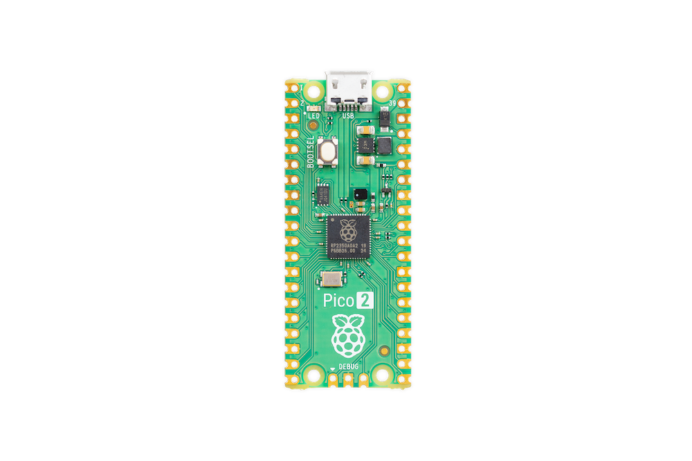
The following diagram shows the pinout of the Pico 2.

At the top of the diagram, you can see that GP25 is connected to the LED, which is why we’re integrating with that pin.

• embassy_rp::init() initializes peripherals.
• PIN_25 is the onboard LED on most RP boards.
• We toggle it on and off with set_high() and set_low(), awaiting 500 ms between transitions.

Thanks to Embassy’s async timers, we don’t block the CPU—we yield control and resume when the delay expires. This model is more efficient than spinning in a tight loop or using busy-waits.

Together, these components demonstrate how a memory-safe, modern Rust framework can map cleanly onto a low-level microcontroller like the RP2350—while still giving us full control over boot, layout, and execution.

Deployment

With our firmware built and ready, it’s time to deploy it to the board.

BOOTSEL Mode

The RP2350 (like the RP2040 before it) includes a USB bootloader in ROM. When the chip is reset while holding down a designated BOOTSEL pin (typically attached to a button), it appears to your computer as a USB mass storage device.

To enter BOOTSEL mode:

1. Hold down the BOOTSEL button.
2. Plug the board into your computer via USB.
3. Release the BOOTSEL button.

You should now see a new USB drive appear (e.g., RPI-RP2 or similar).

This is how the chip expects to be flashed—and it doesn’t require any special debugger or hardware.

Flashing with picotool

Instead of manually dragging and dropping .uf2 files, we can use picotool to flash the .elf binary directly from the terminal.

Since we already set up our runner in .cargo/config.toml, flashing is as simple as:

cargo run --release

Under the hood, this runs:

sudo picotool load -u -v -x -t elf target/thumbv8m.main-none-eabihf/release/rp2350_blink

This does several things:

• Uploads the .elf file to the RP2350 over USB.
• Unmounts the device (-u), ensuring no filesystem issues.
• Verifies the flash (-v) and resets the board (-x).

After Flashing

Once the firmware is written:

• The RP2350 exits BOOTSEL mode.
• It reboots and starts executing your code from flash.
• If everything worked, your LED should now blink—congratulations!

You can now iterate quickly by editing your code and running:

cargo run --release

Just remember: if the program crashes or you need to re-flash, you’ll have to manually put the board back into BOOTSEL mode again.

Conclusion

The RP2350 is a bold step forward in Raspberry Pi’s microcontroller line—combining increased performance, modern security features, and the unique flexibility of dual-architecture support. It’s early days, but the tooling is already solid, and frameworks like Embassy make it approachable even with cutting-edge hardware.

In this post, we set up a full async Rust development environment, explored the RP2350’s memory layout and boot expectations, and flashed a simple—but complete—LED blink program to the board.

If you’ve made it this far: well done! You’ve now got a solid foundation for exploring more advanced features—from PIO and USB to TrustZone and dual-core concurrency.