Creating a Simple Ray Tracer in Haskell

17 Oct 2024

Introduction

Ray tracing is a technique for generating an image by tracing the path of light as pixels in an image plane. It simulates how rays of light interact with objects in a scene to produce realistic lighting, reflections, and shadows.

In this post, we’ll walk through building a simple raytracer in Haskell. We will start with basic vector math, define shapes like spheres and cubes, and trace rays through the scene to generate an image. By the end, you’ll have a raytracer that can render reflections and different shapes.

What You’ll Learn:

Basics of raytracing and the math behind it
How to define math primitives in Haskell
How to trace rays against shapes (including spheres and cubes)
How to generate an image from the traced rays
… a little math

Some Math Primitives

To begin, we need to define some basic 3D vector math. This is essential for all calculations involved in ray tracing: adding vectors, calculating dot products, normalizing vectors, and more.

We’ll define a Vec3 data type to represent 3D vectors and functions for common vector operations.

-- Define a vector (x, y, z) and basic operations
data Vec3 = Vec3 { x :: Double, y :: Double, z :: Double }
deriving (Show, Eq)

-- Vector addition
add :: Vec3 -> Vec3 -> Vec3
add (Vec3 x1 y1 z1) (Vec3 x2 y2 z2) = Vec3 (x1 + x2) (y1 + y2) (z1 + z2)

-- Vector subtraction
sub :: Vec3 -> Vec3 -> Vec3
sub (Vec3 x1 y1 z1) (Vec3 x2 y2 z2) = Vec3 (x1 - x2) (y1 - y2) (z1 - z2)

-- Scalar multiplication
scale :: Double -> Vec3 -> Vec3
scale a (Vec3 x1 y1 z1) = Vec3 (a * x1) (a * y1) (a * z1)

-- Dot product
dot :: Vec3 -> Vec3 -> Double
dot (Vec3 x1 y1 z1) (Vec3 x2 y2 z2) = x1 * x2 + y1 * y2 + z1 * z2

-- Normalize a vector
normalize :: Vec3 -> Vec3
normalize v = scale (1 / len v) v

-- Vector length
len :: Vec3 -> Double
len (Vec3 x1 y1 z1) = sqrt (x1 * x1 + y1 * y1 + z1 * z1)

-- Reflect a vector v around the normal n
reflect :: Vec3 -> Vec3 -> Vec3
reflect v n = sub v (scale (2 * dot v n) n)

Defining a Ray

The ray is the primary tool used to “trace” through the scene, checking for intersections with objects like spheres or cubes.

A ray is defined by its origin \(O\) and direction \(D\). The parametric equation of a ray is:

\[P(t) = O + t \cdot D\]

Where:

\(O\) is the origin
\(D\) is the direction of the ray
\(t\) is a parameter that defines different points along the ray

-- A Ray with an origin and direction
data Ray = Ray { origin :: Vec3, direction :: Vec3 }
    deriving (Show, Eq)

Shapes

To trace rays against objects in the scene, we need to define the concept of a Shape. In Haskell, we’ll use a typeclass to represent different types of shapes (such as spheres and cubes). The Shape typeclass will define methods for calculating ray intersections and normals at intersection points.

ExistentialQuantification and Why We Need It

In Haskell, lists must contain elements of the same type. Since we want a list of various shapes (e.g., spheres and cubes), we need a way to store different shapes in a homogeneous list. We achieve this by using existential quantification to wrap each shape into a common ShapeWrapper.

{-# LANGUAGE ExistentialQuantification #-}

-- Shape typeclass
class Shape a where
    intersect :: Ray -> a -> Maybe Double
    normalAt :: a -> Vec3 -> Vec3
    getColor :: a -> Color
    getReflectivity :: a -> Double

-- A wrapper for any shape that implements the Shape typeclass
data ShapeWrapper = forall a. Shape a => ShapeWrapper a

-- Implement the Shape typeclass for ShapeWrapper
instance Shape ShapeWrapper where
    intersect ray (ShapeWrapper shape) = intersect ray shape
    normalAt (ShapeWrapper shape) = normalAt shape
    getColor (ShapeWrapper shape) = getColor shape
    getReflectivity (ShapeWrapper shape) = getReflectivity shape

Sphere

Sphere Equation

A sphere with center \(C = (c_x, c_y, c_z)\) and radius \(r\) satisfies the equation:

\[(x - c_x)^2 + (y - c_y)^2 + (z - c_z)^2 = r^2\]

In vector form:

\[\lVert P - C \rVert^2 = r^2\]

Where \(P\) is any point on the surface of the sphere, and \(\lVert P - C \rVert\) is the Euclidean distance between \(P\) and the center \(C\).

Substituting the Ray into the Sphere Equation

We substitute the ray equation into the sphere equation:

\[\lVert O + t \cdot D - C \rVert^2 = r^2\]

Expanding this gives:

\[(O + t \cdot D - C) \cdot (O + t \cdot D - C) = r^2\]

Let \(L = O - C\), the vector from the ray origin to the sphere center:

\[(L + t \cdot D) \cdot (L + t \cdot D) = r^2\]

Expanding further:

\[L \cdot L + 2t(L \cdot D) + t^2(D \cdot D) = r^2\]

This is a quadratic equation in \(t\):

\[t^2(D \cdot D) + 2t(L \cdot D) + (L \cdot L - r^2) = 0\]

Solving the Quadratic Equation

The equation can be solved using the quadratic formula:

\[t = \frac{-b \pm \sqrt{b^2 - 4ac}}{2a}\]

Where:

a is defined as: \(a = D \cdot D\)
b is defined as: \(b = 2(L \cdot D)\)
c is defined as: \(c = L \cdot L - r^2\)

The discriminant \(\Delta = b^2 - 4ac\) determines the number of intersections:

\(\Delta < 0\): no intersection
\(\Delta = 0\): tangent to the sphere
\(\Delta > 0\): two intersection points

Here’s how we define a Sphere as a Shape with a center, radius, color, and reflectivity.

-- A Sphere with a center, radius, color, and reflectivity
data Sphere = Sphere { center :: Vec3, radius :: Double, sphereColor :: Color, sphereReflectivity :: Double }
    deriving (Show, Eq)

instance Shape Sphere where
    intersect (Ray o d) (Sphere c r _ _) =
        let oc = sub o c
        a = dot d d
        b = 2.0 * dot oc d
        c' = dot oc oc - r * r
        discriminant = b * b - 4 * a * c'
        in if discriminant < 0
        then Nothing
        else Just ((-b - sqrt discriminant) / (2.0 * a))

    normalAt (Sphere c _ _ _) p = normalize (sub p c)
    getColor (Sphere _ _ color _) = color
    getReflectivity (Sphere _ _ _ reflectivity) = reflectivity

Cube Definition

For a cube, we typically use an axis-aligned bounding box (AABB), which means the cube’s faces are aligned with the coordinate axes. The problem of ray-cube intersection becomes checking where the ray crosses the planes of the box’s sides.

The cube can be defined by two points: the minimum corner \(\text{minCorner} = (x_{\text{min}}, y_{\text{min}}, z_{\text{min}})\) and the maximum corner \(\text{maxCorner} = (x_{\text{max}}, y_{\text{max}}, z_{\text{max}})\). The intersection algorithm involves calculating for each axis independently and then combining the results.

Cube Planes and Ray Intersections

For each axis (x, y, z), the cube has two planes: one at the minimum bound and one at the maximum bound. The idea is to calculate the intersections of the ray with each of these planes.

For the x-axis, for example, we compute the parameter \(t\) where the ray hits the two x-planes:

\[t_{\text{min}, x} = \frac{x_{\text{min}} - O_x}{D_x}\] \[t_{\text{max}, x} = \frac{x_{\text{max}} - O_x}{D_x}\]

We do the same for the y-axis and z-axis:

\[t_{\text{min}, y} = \frac{y_{\text{min}} - O_y}{D_y}\] \[t_{\text{max}, y} = \frac{y_{\text{max}} - O_y}{D_y}\] \[t_{\text{min}, z} = \frac{z_{\text{min}} - O_z}{D_z}\] \[t_{\text{max}, z} = \frac{z_{\text{max}} - O_z}{D_z}\]

Combining the Results

The idea is to calculate when the ray enters and exits the cube. The entry point is determined by the maximum of the \(t_{\text{min}}\) values across all axes (because the ray must enter the cube from the farthest plane), and the exit point is determined by the minimum of the \(t_{\text{max}}\) values across all axes (because the ray must exit at the nearest plane):

\[t_{\text{entry}} = \max(t_{\text{min}, x}, t_{\text{min}, y}, t_{\text{min}, z})\] \[t_{\text{exit}} = \min(t_{\text{max}, x}, t_{\text{max}, y}, t_{\text{max}, z})\]

If \(t_{\text{entry}} > t_{\text{exit}}\) or \(t_{\text{exit}} < 0\), the ray does not intersect the cube.

Final Cube Intersection Condition

To summarize, the cube-ray intersection works as follows:

Calculate \(t_{\text{min}}\) and \(t_{\text{max}}\) for each axis.
Compute the entry and exit points.
If the entry point occurs after the exit point (or both are behind the ray origin), there is no intersection.

-- A Cube defined by its minimum and maximum corners
data Cube = Cube { minCorner :: Vec3, maxCorner :: Vec3, cubeColor :: Color, cubeReflectivity :: Double }
deriving (Show, Eq)

instance Shape Cube where
    intersect (Ray o d) (Cube (Vec3 xmin ymin zmin) (Vec3 xmax ymax zmax) _ _) =
        let invD = Vec3 (1 / x d) (1 / y d) (1 / z d)
        t0 = (Vec3 xmin ymin zmin `sub` o) `mul` invD
        t1 = (Vec3 xmax ymax zmax `sub` o) `mul` invD
        tmin = maximum [minimum [x t0, x t1], minimum [y t0, y t1], minimum [z t0, z t1]]
        tmax = minimum [maximum [x t0, x t1], maximum [y t0, y t1], maximum [z t0, z t1]]
        in if tmax < tmin || tmax < 0 then Nothing else Just tmin

    normalAt (Cube (Vec3 xmin ymin zmin) (Vec3 xmax ymax zmax) _ _) p =
        let (Vec3 px py pz) = p
        in if abs (px - xmin) < 1e-4 then Vec3 (-1) 0 0
           else if abs (px - xmax) < 1e-4 then Vec3 1 0 0
           else if abs (py - ymin) < 1e-4 then Vec3 0 (-1) 0
           else if abs (py - ymax) < 1e-4 then Vec3 0 1 0
           else if abs (pz - zmin) < 1e-4 then Vec3 0 0 (-1)
           else Vec3 0 0 1

    getColor (Cube _ _ color _) = color

    getReflectivity (Cube _ _ _ reflectivity) = reflectivity

Tracing a Ray Against Scene Objects

Once we have rays and shapes, we can start tracing rays through the scene. The traceRay function checks each ray against all objects in the scene and calculates the color at the point where the ray intersects an object.

-- Maximum recursion depth for reflections
maxDepth :: Int
maxDepth = 5

-- Trace a ray in the scene, returning the color with reflections
traceRay :: [ShapeWrapper] -> Ray -> Int -> Color
traceRay shapes ray depth
    | depth >= maxDepth = Vec3 0 0 0  -- If we reach the max depth, return black (no more reflections)
    | otherwise = case closestIntersection of
        Nothing -> backgroundColor  -- No intersection, return background color
        Just (shape, t) -> let hitPoint = add (origin ray) (scale t (direction ray))
                               normal = normalAt shape hitPoint
                               reflectedRay = Ray hitPoint (reflect (direction ray) normal)
                               reflectionColor = traceRay shapes reflectedRay (depth + 1)
                               objectColor = getColor shape
                           in add (scale (1 - getReflectivity shape) objectColor)
                                  (scale (getReflectivity shape) reflectionColor)
    where
        intersections = [(shape, dist) | shape <- shapes, Just dist <- [intersect ray shape]]
        closestIntersection = if null intersections 
                              then Nothing 
                              else Just $ minimumBy (comparing snd) intersections
        backgroundColor = Vec3 0.5 0.7 1.0  -- Sky blue background

Putting It All Together

We can now render a scene by tracing rays for each pixel and writing the output to an image file in PPM format.

-- Create a ray from the camera to the pixel at (u, v)
getRay :: Double -> Double -> Ray
getRay u v = Ray (Vec3 0 0 0) (normalize (Vec3 u v (-1)))

-- Render the scene
render :: Int -> Int -> [ShapeWrapper] -> [[Color]]
render width height shapes =
    [[traceRay shapes (getRay (2 * (fromIntegral x / fromIntegral width) - 1)
                              (2 * (fromIntegral y / fromIntegral height) - 1)) 0
      | x <- [0..width-1]]
      | y <- [0..height-1]]

-- Convert a color to an integer pixel value (0-255)
toColorInt :: Color -> (Int, Int, Int)
toColorInt (Vec3 r g b) = (floor (255.99 * clamp r), floor (255.99 * clamp g), floor (255.99 * clamp b))
    where clamp x = max 0.0 (min 1.0 x)

-- Output the image in PPM format
writePPM :: FilePath -> [[Color]] -> IO ()
writePPM filename image = writeFile filename $ unlines $
    ["P3", show width ++ " " ++ show height, "255"] ++
    [unwords [show r, show g, show b] | row <- image, (r, g, b) <- map toColorInt row]
    where
        height = length image
        width = length (head image)

Examples

Here’s an example where we render two spheres and a cube:

main :: IO ()
main = do
    let width = 1024
    height = 768
    shapes = [ ShapeWrapper (Sphere (Vec3 (-1.0) 0 (-1)) 0.5 (Vec3 0.8 0.3 0.3) 0.5),  -- Red sphere
               ShapeWrapper (Sphere (Vec3 1 0 (-1)) 0.5 (Vec3 0.3 0.8 0.3) 0.5),       -- Green sphere
               ShapeWrapper (Cube (Vec3 (-0.5) (-0.5) (-2)) (Vec3 0.5 0.5 (-1.5)) (Vec3 0.8 0.8 0.0) 0.5)  -- Yellow cube
             ]
    image = render width height shapes
    writePPM "output.ppm" image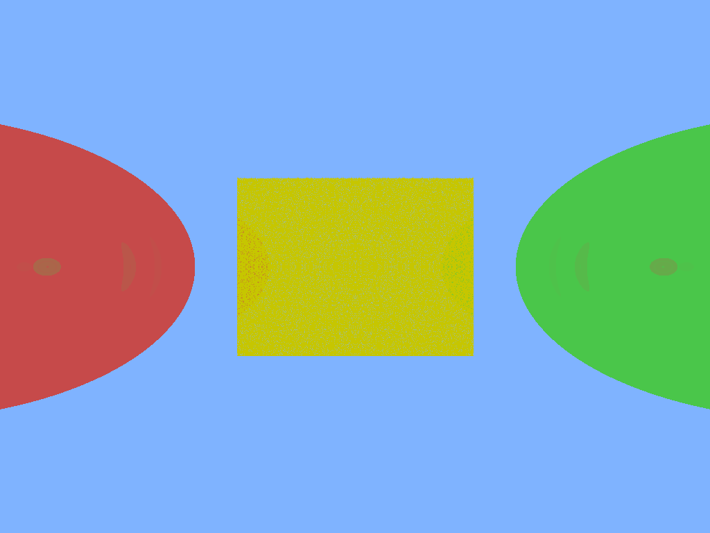

Simple Scene

Conclusion

In this post, we’ve built a simple raytracer in Haskell that supports basic shapes like spheres and cubes. You can extend this to add more complex features like shadows, lighting models, and textured surfaces. Happy ray tracing!

The full code is available here as a gist:

Cogs and Levers A blog full of technical stuff