Perlin Noise

Introduction

Noise functions in computer applications allow programmers to make the machine act a little more naturally. It’s the randomness introduced with these algorithms that gives the computer what appears to be “free thought” or unexpected decisions.

Today, I’ll walk through the Perlin Noise algorithm which has applications in computer science ranging from player movement, landscape generation, clouds, etc.

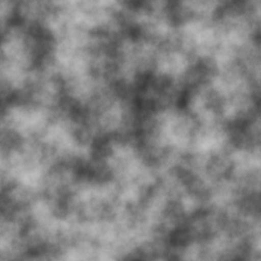
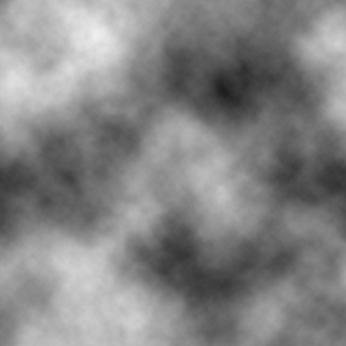
Here are some examples of the Perlin Noise function output into two dimensions:

In today’s post, I’ll walk through the Perlin Noise algorithm and what steps you need to take to implement it yourself.

Understanding Noise

The Perlin Noise algorithm can be broken down into a few smaller pieces to make it easier to understand. At its heart, the algorithm needs pseudo-random numbers. These random numbers should be repeatable so that you can re-generate the same noise pattern at will.

A common noise function for two parameters that I have found used over the web is as follows:

float noise(const int x, const int y) {
  int n = x + y * 57;
  n = (n << 13) ^ n;
  return (1.0f - ( ( n * (n * n * 15731 + 789221) + 1376312589) & 0x7FFFFFFF) / 1073741824.0f);
}

There’s a lot of math transformation in this previous function. You can use any function at all to produce your random numbers, just make sure that you can generate them against two parameters (in the case of 2d) and that you’ll get repeatable results.

Next we’ll smooth out the noise between two points. We’ll do this by sampling the corners, sides and centre of the point we’re currently generating for.

float smoothNoise(const float x, const float y) {
  int ix = (int)x;
  int iy = (int)y;

  // sample the corners
  float corners = (noise(ix - 1, iy - 1) +
                   noise(ix + 1, iy - 1) +
                   noise(ix - 1, iy + 1) +
                   noise(ix + 1, iy + 1)) / 16;

  // sample the sides
  float sides = (noise(ix - 1, iy) +
                 noise(ix + 1, iy) +
                 noise(ix, iy - 1) +
                 noise(ix, iy + 1)) / 8;

  // sample the centre
  float centre = noise(ix, iy);

  // send out the accumulated result
  return corners + sides + centre;
}

With the above function, we can now sample a small area for a given point. All based on our random number generator.

For the fractional parts that occur between solid boundaries, we’ll use a specific interpolation method. I’ve defined two below. One that will do linear interpolation and one that will use cosine for a smoother transition between points.

/* Linear interpolation */
float lerp(float a, float b, float x) {
   return a * (1 - x) + b * x;
}

/* Trigonometric interpolation */
float terp(float a, float b, float x) {
  float ft = x * 3.1415927f;
  float f = (1 - cosf(ft)) * 0.5f;

  return a * (1 - f) + b * f;
}

/* Noise interpolation */
float interpolateNoise(const float x, const float y) {
  int   ix = (int)x;
  float fx = x - ix;

  int   iy = (int)y;
  float fy = y - iy;

  float v1 = smoothNoise(ix, iy),
        v2 = smoothNoise(ix + 1, iy),
        v3 = smoothNoise(ix, iy + 1),
        v4 = smoothNoise(ix + 1, iy + 1);

  float i1 = terp(v1, v2, fx),
        i2 = terp(v3, v4, fx);

  return terp(i1, i2, fy);
}

Finally we use this smooth interpolation to perform the perlin noise function. A couple of interesting co-effecients that are provided to the algorithm are “octaves” and “persistence”. “octaves” defines how many iterations that will be performed and “persistence” defines how much of the spectrum we’ll utilise. It’s highly interactive to the main curve co-effecients: frequency and amplitude.

float perlin2d(const float x, const float y,
               const int octaves, const float persistence) {
  float total = 0.0f;

  for (int i = 0; i <= (octaves - 1); i ++) {
    float frequency = powf(2, i);
    float amplitude = powf(persistence, i);

    total = total + interpolateNoise(x * frequency, y * frequency) * amplitude;
  }

  return total;
}

This now provides us with a way to create a map (or 2d array) to produce images much like I’d pasted in above. Here is a typical build loop.

for (int x = 0; x < w; x ++) {
  for (int y = 0; y < h; y ++) {
    float xx = (float)x / (float)this->width;
    float yy = (float)y / (float)this->height;

    map[x + (y * w)] = perlin::perlin2d(
      xx, yy,
      6, 1.02f
    );
  }
}

That should be enough to get you going.