Rendering realistic 3D environments is more than just defining surfaces—atmospheric effects like fog, mist, and light
scattering add a layer of depth and realism that makes a scene feel immersive. In this post, we’ll explore volumetric
fog and how we can implement it in our ray-marched Mandelbulb fractal shader.
What is Volumetric Fog?
Volumetric fog is an effect that simulates light scattering through a medium, such as:
Mist over a landscape
Dense fog hiding distant objects
Hazy light beams filtering through an object
Unlike simple screen-space fog, volumetric fog interacts with geometry, light, and depth, making it appear more
natural. In our case, we’ll use it to create a soft, atmospheric effect around our Mandelbulb fractal.
How Does It Work?
Volumetric fog in ray marching is achieved by stepping through the scene and accumulating fog density based on
distance. This is done using:
Exponential Fog – A basic formula that fades objects into the fog over distance.
Light Scattering – Simulates god rays by accumulating light along the ray path.
Procedural Noise Fog – Uses random noise to create a more natural, rolling mist effect.
We’ll build each of these effects step by step, expanding on our existing Mandelbulb shader to enhance its atmosphere.
If you haven’t seen them already, suggested reading are the previous articles in this series:
We will start with the following code, which is our phong shaded, lit, mandelbulb with the camera spinning around it.
floatmandelbulbSDF(vec3pos){vec3z=pos;floatdr=1.0;floatr;constintiterations=8;constfloatpower=8.0;for(inti=0;i<iterations;i++){r=length(z);if(r>2.0)break;floattheta=acos(z.z/r);floatphi=atan(z.y,z.x);floatzr=pow(r,power-1.0);dr=zr*power*dr+1.0;zr*=r;theta*=power;phi*=power;z=zr*vec3(sin(theta)*cos(phi),sin(theta)*sin(phi),cos(theta))+pos;}return0.5*log(r)*r/dr;}vec3getNormal(vec3p){vec2e=vec2(0.001,0.0);returnnormalize(vec3(mandelbulbSDF(p+e.xyy)-mandelbulbSDF(p-e.xyy),mandelbulbSDF(p+e.yxy)-mandelbulbSDF(p-e.yxy),mandelbulbSDF(p+e.yyx)-mandelbulbSDF(p-e.yyx)));}// Basic Phong shadingvec3phongLighting(vec3p,vec3viewDir){vec3normal=getNormal(p);// Light settingsvec3lightPos=vec3(2.0,2.0,-2.0);vec3lightDir=normalize(lightPos-p);vec3ambient=vec3(0.1);// Ambient light// Diffuse lightingfloatdiff=max(dot(normal,lightDir),0.0);// Specular highlightvec3reflectDir=reflect(-lightDir,normal);floatspec=pow(max(dot(viewDir,reflectDir),0.0),16.0);// Shininess factorreturnambient+diff*vec3(1.0,0.8,0.6)+spec*vec3(1.0);// Final color}// Soft Shadows (traces a secondary ray to detect occlusion)floatsoftShadow(vec3ro,vec3rd){floatres=1.0;floatt=0.02;// Small starting stepfor(inti=0;i<24;i++){floatd=mandelbulbSDF(ro+rd*t);if(d<0.001)return0.0;// Fully in shadowres=min(res,10.0*d/t);// Soft transitiont+=d;}returnres;}voidmainImage(outvec4fragColor,invec2fragCoord){vec2uv=(fragCoord-0.5*iResolution.xy)/iResolution.y;// Rotating Camerafloatangle=iTime*0.5;vec3rayOrigin=vec3(3.0*cos(angle),0.0,3.0*sin(angle));vec3target=vec3(0.0);vec3forward=normalize(target-rayOrigin);vec3right=normalize(cross(vec3(0,1,0),forward));vec3up=cross(forward,right);vec3rayDir=normalize(forward+uv.x*right+uv.y*up);// Ray marchingfloattotalDistance=0.0;constintmaxSteps=100;constfloatminDist=0.001;constfloatmaxDist=10.0;vec3hitPoint;for(inti=0;i<maxSteps;i++){hitPoint=rayOrigin+rayDir*totalDistance;floatdist=mandelbulbSDF(hitPoint);if(dist<minDist)break;if(totalDistance>maxDist)break;totalDistance+=dist;}// Compute lighting only if we hit the fractalvec3color;if(totalDistance<maxDist){vec3viewDir=normalize(rayOrigin-hitPoint);vec3baseLight=phongLighting(hitPoint,viewDir);floatshadow=softShadow(hitPoint,normalize(vec3(2.0,2.0,-2.0)));color=baseLight*shadow;// Apply shadows}else{color=vec3(0.1,0.1,0.2);// Background color}fragColor=vec4(color,1.0);}
Depth-based Blending
To create a realistic sense of depth, we can use depth-based blending to gradually fade objects into the fog as they
move further away from the camera. This simulates how light scatters in the atmosphere, making distant objects appear
less distinct.
In ray marching, we calculate fog intensity using exponential depth functions like:
where distance is how far along the ray we’ve traveled, and densityFactor controls how quickly objects fade into
fog.
By blending our object’s color with the fog color based on this function, we achieve a smooth atmospheric fade effect.
Let’s implement it in our shader.
voidmainImage(outvec4fragColor,invec2fragCoord){vec2uv=(fragCoord-0.5*iResolution.xy)/iResolution.y;// Rotating Camerafloatangle=iTime*0.5;vec3rayOrigin=vec3(3.0*cos(angle),0.0,3.0*sin(angle));vec3target=vec3(0.0);vec3forward=normalize(target-rayOrigin);vec3right=normalize(cross(vec3(0,1,0),forward));vec3up=cross(forward,right);vec3rayDir=normalize(forward+uv.x*right+uv.y*up);// Ray marchingfloattotalDistance=0.0;constintmaxSteps=100;constfloatminDist=0.001;constfloatmaxDist=10.0;vec3hitPoint;for(inti=0;i<maxSteps;i++){hitPoint=rayOrigin+rayDir*totalDistance;floatdist=mandelbulbSDF(hitPoint);if(dist<minDist)break;if(totalDistance>maxDist)break;totalDistance+=dist;}// Compute lighting only if we hit the fractalvec3color;if(totalDistance<maxDist){vec3viewDir=normalize(rayOrigin-hitPoint);vec3baseLight=phongLighting(hitPoint,viewDir);floatshadow=softShadow(hitPoint,normalize(vec3(2.0,2.0,-2.0)));color=baseLight*shadow;}else{color=vec3(0.1,0.1,0.2);// Background color}// Apply depth-based exponential fogfloatfogAmount=1.0-exp(-totalDistance*0.15);color=mix(color,vec3(0.5,0.6,0.7),fogAmount);fragColor=vec4(color,1.0);}
Once this is running, you should see some fog appear to obscure our Mandelbulb:
Light Scattering
When light passes through a medium like fog, dust, or mist, it doesn’t just stop—it scatters in different directions,
creating beautiful effects like god rays or a soft glow around objects. This is known as volumetric light scattering.
In ray marching, we can approximate this effect by tracing secondary rays through the scene and accumulating light
contribution along the path. The more dense the medium (or the more surfaces the ray encounters), the stronger the
scattering effect. A simplified formula for this accumulation looks like:
You can see the god rays through the centre of our fractal:
With this code we’ve:
Shot a secondary ray into the scene which accumulates scattered light
The denser the fractal, the more light it scatters
density += 0.02 controls the intensity of the god rays
Noise-based Fog
Real-world fog isn’t uniform—it swirls, shifts, and forms dense or sparse patches. To create a more natural effect, we
can use procedural noise to simulate rolling mist or dynamic fog layers.
Instead of applying a constant fog density at every point, we introduce random variations using a noise function:
\(\text{fogDensity}(p)\) determines the fog’s thickness at position \(p\).
\(\text{baseDensity}\) is the overall fog intensity.
\(\text{noise}(p)\) generates small-scale variations to make fog look natural.
By sampling noise along the ray, we can create wispy, uneven fog that behaves more like mist or smoke, enhancing the
realism of our scene. Let’s implement this effect next.
We’ll add procedural noise to simulate smoke or rolling mist.
After these modifications, you should start to see the fog moving as we rotate:
The final version of this shader can be found here.
Conclusion
By adding volumetric effects to our ray-marched Mandelbulb, we’ve taken our scene from a simple fractal to a rich,
immersive environment.
These techniques not only enhance the visual depth of our scene but also provide a foundation for more advanced
effects like clouds, smoke, fire, or atmospheric light absorption.
Ray tracing is known for producing stunning reflections, we can achieve the same effect using ray
marching. In this post, we’ll walk through a classic two-sphere reflective scene, but instead of traditional ray
tracing, we’ll ray march our way to stunning reflections.
The first step is defining a scene with two spheres and a ground plane. In ray marching, objects are defined using
signed distance functions (SDFs). Our scene SDF is just a combination of smaller SDFs.
SDFs
The SDF for a sphere gives us the distance from any point to the surface of the sphere:
Now we trace a ray through our scene using ray marching.
vec3rayMarch(vec3rayOrigin,vec3rayDir,intmaxSteps,floatmaxDist){floattotalDistance=0.0;vec3hitPoint;for(inti=0;i<maxSteps;i++){hitPoint=rayOrigin+rayDir*totalDistance;floatdist=sceneSDF(hitPoint);if(dist<0.001)break;// Close enough to surfaceif(totalDistance>maxDist)returnvec3(0.5,0.7,1.0);// Sky colortotalDistance+=dist;}returnhitPoint;// Return the hit location}
Surface Normals
For lighting and reflections, we need surface normals. These are estimated using small offsets in each direction:
voidmainImage(outvec4fragColor,invec2fragCoord){vec2uv=(fragCoord-0.5*iResolution.xy)/iResolution.y;// Camera Setupvec3rayOrigin=vec3(0,0,-5);vec3rayDir=normalize(vec3(uv,1.0));// Perform Ray Marchingvec3hitPoint=rayMarch(rayOrigin,rayDir,100,10.0);// If we hit an object, apply shadingvec3color;if(hitPoint!=vec3(0.5,0.7,1.0)){vec3viewDir=normalize(rayOrigin-hitPoint);vec3baseLight=phongLighting(hitPoint,viewDir);vec3reflection=computeReflection(hitPoint,rayDir);color=mix(baseLight,reflection,0.5);// Blend reflections}else{color=vec3(0.5,0.7,1.0);// Sky color}fragColor=vec4(color,1.0);}
Running this shader, you should see two very reflective spheres reflecting each other.
Conclusion
With just a few functions, we’ve recreated a classic ray tracing scene using ray marching. This technique allows
us to:
Render reflective surfaces without traditional ray tracing
Generate soft shadows using SDF normals
Extend the method for refraction and more complex materials
Fractals are some of the most mesmerizing visuals in computer graphics, but rendering them in 3D space requires
special techniques beyond standard polygonal rendering. This article will take you into the world of ray marching,
where we’ll use distance fields, lighting, and soft shadows to render a Mandelbulb fractal — one of the most famous 3D
fractals.
By the end of this post, you’ll understand:
The basics of ray marching and signed distance functions (SDFs).
How to render 3D objects without polygons.
How to implement Phong shading for realistic lighting.
How to compute soft shadows for better depth.
How to animate a rotating Mandelbulb fractal.
This article will build on the knowledge that we established in the Basics of Shader Programming
article that we put together earlier. If you haven’t read through that one, it’ll be worth taking a look at.
What is Ray Marching?
Ray marching is a distance-based rendering technique that is closely related to ray tracing.
However, instead of tracing rays until they hit exact geometry (like in traditional ray tracing), ray marching steps
along the ray incrementally using distance fields.
Each pixel on the screen sends out a ray into 3D space. We then march forward along the ray, using a signed
distance function (SDF) to tell us how far we are from the nearest object. This lets us render smooth implicit
surfaces like fractals and organic shapes.
Our first SDF
The simplest 3D object we can render using ray marching is a sphere. We define its shape using a
signed distance function (SDF):
// Sphere Signed Distance Function (SDF)floatsdfSphere(vec3p,floatr){returnlength(p)-r;}
The sdfSphere() function returns the shortest distance from any point in space to the sphere’s surface.
We can now step along that ray until we reach the sphere. We do this by integrating our sfpSphere() function into our
mainImage() function:
voidmainImage(outvec4fragColor,invec2fragCoord){vec2uv=(fragCoord-0.5*iResolution.xy)/iResolution.y;// Camera setupvec3rayOrigin=vec3(0,0,-3);vec3rayDir=normalize(vec3(uv,1));floattotalDistance=0.0;constintmaxSteps=100;constfloatminDist=0.001;constfloatmaxDist=20.0;for(inti=0;i<maxSteps;i++){vec3pos=rayOrigin+rayDir*totalDistance;floatdist=sdfSphere(pos,1.0);if(dist<minDist)break;if(totalDistance>maxDist)break;totalDistance+=dist;}vec3col=(totalDistance<maxDist)?vec3(1.0):vec3(0.2,0.3,0.4);fragColor=vec4(col,1.0);}
First of all here, we convert the co-ordinate that we’re processing into screen co-ordinates:
We now iterate (march) down the ray to a maximum of maxSteps (currently set to 100) to determine if the ray
intersects with our sphere (via sdfSphere).
Finally, we render the colour of our sphere if the distance is within tolerance; otherwise we consider this part of
the background:
In order to make this sphere look a little more 3D, we can light it. In order to light any object, we need to be able
to compute surface normals. We do that via a function like this:
vec3getNormal(vec3p){vec2e=vec2(0.001,0.0);// Small offset for numerical differentiationreturnnormalize(vec3(sdfSphere(p+e.xyy,1.0)-sdfSphere(p-e.xyy,1.0),sdfSphere(p+e.yxy,1.0)-sdfSphere(p-e.yxy,1.0),sdfSphere(p+e.yyx,1.0)-sdfSphere(p-e.yyx,1.0)));}
We make decisions about the actual colour via a lighting function. This lighting function is informed by the surface
normals that it computes:
vec3lighting(vec3p){vec3lightPos=vec3(2.0,2.0,-2.0);// Light source positionvec3normal=getNormal(p);// Compute the normal at point 'p'vec3lightDir=normalize(lightPos-p);// Direction to lightfloatdiff=max(dot(normal,lightDir),0.0);// Diffuse lightingreturnvec3(diff);// Return grayscale lighting effect}
We can now integrate this back into our scene in the mainImage function. Rather than just making a static colour
return when we establish a hit point, we start to execute the lighting function towards the end of the function:
voidmainImage(outvec4fragColor,invec2fragCoord){vec2uv=(fragCoord-0.5*iResolution.xy)/iResolution.y;// Camera setupvec3rayOrigin=vec3(0,0,-3);// Camera positioned at (0,0,-3)vec3rayDir=normalize(vec3(uv,1));// Forward-facing ray// Ray marching parametersfloattotalDistance=0.0;constintmaxSteps=100;constfloatminDist=0.001;constfloatmaxDist=20.0;vec3hitPoint;// Ray marching loopfor(inti=0;i<maxSteps;i++){hitPoint=rayOrigin+rayDir*totalDistance;floatdist=sdfSphere(hitPoint,1.0);// Distance to the sphereif(dist<minDist)break;// If we are close enough to the surface, stopif(totalDistance>maxDist)break;// If we exceed max distance, stoptotalDistance+=dist;}// If we hit something, apply shading; otherwise, keep background colorvec3col=(totalDistance<maxDist)?lighting(hitPoint):vec3(0.2,0.3,0.4);fragColor=vec4(col,1.0);}
You should see something similar to this:
Mandelbulbs
We can now upgrade our rendering to use something a little more complex then our sphere.
SDF
The Mandelbulb is a 3D fractal inspired by the 2D Mandelbrot Set. Instead of working in 2D complex numbers, it uses
spherical coordinates in 3D space.
The core formula: \(z→zn+c\) is extended to 3D using spherical math.
Instead of a sphere SDF, we’ll use an iterative function to compute distances to the fractal surface.
This function iterates over complex numbers in 3D space to compute the Mandelbulb structure.
Raymarching the Mandelbulb
Now, we can take a look at what this produces. We use our newly created SDF to get our hit point. We’ll use this
distance value as well to establish different colours.
voidmainImage(outvec4fragColor,invec2fragCoord){vec2uv=(fragCoord-0.5*iResolution.xy)/iResolution.y;// Camera setupvec3rayOrigin=vec3(0,0,-4);vec3rayDir=normalize(vec3(uv,1));// Ray marching parametersfloattotalDistance=0.0;constintmaxSteps=100;constfloatminDist=0.001;constfloatmaxDist=10.0;vec3hitPoint;// Ray marching loopfor(inti=0;i<maxSteps;i++){hitPoint=rayOrigin+rayDir*totalDistance;floatdist=mandelbulbSDF(hitPoint);// Fractal distance functionif(dist<minDist)break;if(totalDistance>maxDist)break;totalDistance+=dist;}// Color based on distance (simple shading)vec3col=(totalDistance<maxDist)?vec3(1.0-totalDistance*0.1):vec3(0.1,0.1,0.2);fragColor=vec4(col,1.0);}
You should see something similar to this:
Rotation
We can’t see much with how this object is oriented. By adding some basic animation, we can start to look at the complexities
of how this object is put together. We use the global iTime variable here to establish movement:
voidmainImage(outvec4fragColor,invec2fragCoord){vec2uv=(fragCoord-0.5*iResolution.xy)/iResolution.y;// Rotate camera around the fractal using iTimefloatangle=iTime*0.5;// Adjust speed of rotationvec3rayOrigin=vec3(3.0*cos(angle),0.0,3.0*sin(angle));// Circular pathvec3target=vec3(0.0,0.0,0.0);// Looking at the fractalvec3forward=normalize(target-rayOrigin);vec3right=normalize(cross(vec3(0,1,0),forward));vec3up=cross(forward,right);vec3rayDir=normalize(forward+uv.x*right+uv.y*up);// Ray marching parametersfloattotalDistance=0.0;constintmaxSteps=100;constfloatminDist=0.001;constfloatmaxDist=10.0;vec3hitPoint;// Ray marching loopfor(inti=0;i<maxSteps;i++){hitPoint=rayOrigin+rayDir*totalDistance;floatdist=mandelbulbSDF(hitPoint);// Fractal distance functionif(dist<minDist)break;if(totalDistance>maxDist)break;totalDistance+=dist;}// Color based on distance (simple shading)vec3col=(totalDistance<maxDist)?vec3(1.0-totalDistance*0.1):vec3(0.1,0.1,0.2);fragColor=vec4(col,1.0);}
You should see something similar to this:
Lights
In order to make our fractal look 3D, we need to be able to compute our surface normals. We’ll be using the
mandelbulbSDF function above to accomplish this:
To make the fractal look more realistic, we’ll implement soft shadows. This will really enhance how this object looks.
// Soft Shadows (traces a secondary ray to detect occlusion)floatsoftShadow(vec3ro,vec3rd){floatres=1.0;floatt=0.02;// Small starting stepfor(inti=0;i<24;i++){floatd=mandelbulbSDF(ro+rd*t);if(d<0.001)return0.0;// Fully in shadowres=min(res,10.0*d/t);// Soft transitiont+=d;}returnres;}
Pulling it all together
We can now pull all of these enhancements together with our main image function:
voidmainImage(outvec4fragColor,invec2fragCoord){vec2uv=(fragCoord-0.5*iResolution.xy)/iResolution.y;// Rotating Camerafloatangle=iTime*0.5;vec3rayOrigin=vec3(3.0*cos(angle),0.0,3.0*sin(angle));vec3target=vec3(0.0);vec3forward=normalize(target-rayOrigin);vec3right=normalize(cross(vec3(0,1,0),forward));vec3up=cross(forward,right);vec3rayDir=normalize(forward+uv.x*right+uv.y*up);// Ray marchingfloattotalDistance=0.0;constintmaxSteps=100;constfloatminDist=0.001;constfloatmaxDist=10.0;vec3hitPoint;for(inti=0;i<maxSteps;i++){hitPoint=rayOrigin+rayDir*totalDistance;floatdist=mandelbulbSDF(hitPoint);if(dist<minDist)break;if(totalDistance>maxDist)break;totalDistance+=dist;}// Compute lighting only if we hit the fractalvec3color;if(totalDistance<maxDist){vec3viewDir=normalize(rayOrigin-hitPoint);vec3baseLight=phongLighting(hitPoint,viewDir);floatshadow=softShadow(hitPoint,normalize(vec3(2.0,2.0,-2.0)));color=baseLight*shadow;// Apply shadows}else{color=vec3(0.1,0.1,0.2);// Background color}fragColor=vec4(color,1.0);}
Finally, you should see something similar to this:
Shaders are one of the most powerful tools in modern computer graphics, allowing real-time effects, lighting, and
animation on the GPU (Graphics Processing Unit). They are used in games, simulations, and rendering engines
to control how pixels and geometry appear on screen.
In this article, we’ll break down:
What shaders are and why they matter
How to write your first shader
Understanding screen coordinates
Animating a shader
This guide assumes zero prior knowledge of shaders and will explain each line of code step by step.
All of the code here can be run using Shadertoy. You won’t need to install any dependencies,
but you will need a GPU-capable computer!
What is a Shader?
A shader is a small program that runs on the GPU. Unlike regular CPU code, shaders are executed in parallel for
every pixel or vertex on the screen.
Types of Shaders
Vertex Shader – Moves and transforms individual points in 3D space.
Fragment Shader (Pixel Shader) – Determines the final color of each pixel.
For now, we’ll focus on fragment shaders since they control how things look.
Your First Shader
Let’s start with the simplest shader possible: a solid color fill.
Seeing Red!
voidmainImage(outvec4fragColor,invec2fragCoord){fragColor=vec4(1.0,0.0,0.0,1.0);// Solid red color}
Breaking this code down:
void mainImage(...) → This function runs for every pixel on the screen.
fragColor → The output color of the pixel.
vec4(1.0, 0.0, 0.0, 1.0) → This defines an RGBA color:
1.0, 0.0, 0.0 → Red
1.0 → Fully opaque (no transparency)
Try This: Change the color values:
vec4(0.0, 1.0, 0.0, 1.0); → Green
vec4(0.0, 0.0, 1.0, 1.0); → Blue
vec4(1.0, 1.0, 0.0, 1.0); → Yellow
Mapping Colors to Screen Position
Instead of filling the screen with a single color, let’s map colors to pixel positions.
A Gradient Shader
voidmainImage(outvec4fragColor,invec2fragCoord){vec2uv=fragCoord/iResolution.xy;// Normalize coordinates (0 to 1)fragColor=vec4(uv.x,uv.y,0.5,1.0);}
Breaking this code down:
fragCoord / iResolution.xy → Converts pixel coordinates into a 0 → 1 range.
uv.x → Controls red (left to right gradient).
uv.y → Controls green (bottom to top gradient).
0.5 → Keeps blue constant.
This creates a smooth gradient across the screen!
Try This: Swap uv.x and uv.y to see different patterns.
Animation
Shaders can react to time using iTime. This lets us create dynamic effects.
sin(uv.x * 10.0 + iTime) → Creates waves that move over time.
The whole screen pulses from black to white dynamically.
Try This: Change 10.0 to 20.0 or 5.0 to make waves tighter or wider.
Wrapping up
Here have been some very simple shader programs to get started with. In future articles, we’ll build on this knowledge
to build more exciting graphics applications.
Radio signals surround us every day—whether it’s FM radio in your car, WiFi on your laptop, or Bluetooth connecting
your phone to wireless headphones. These signals are all based on the same fundamental principles: frequency,
modulation, and bandwidth.
In today’s article, I want to go through some of the fundamentals:
How do radio signals travel through the air?
What is the difference between AM and FM?
How can multiple signals exist without interfering?
What is digital modulation (FSK & PSK), and why does it matter?
How can we capture and transmit signals using HackRF?
By the end of this article, we should be running some experiments with our own software defined radio devices.
Getting Setup
Before getting started in this next section, you’ll want to make sure that you have some specific software installed
on your computer, as well as a software defined radio device.
I’m using a HackRF One as my device of choice as it integrates with all of
the software that I use.
Make sure you have the following packages installed:
hackrf
gqrx
gnuradio
sudo pacman -S hackrf gqrx gnuradio
Create yourself a new python project and virtual environment, and install the libraries that will wrap some of these
tools to give you an easy to use programming environment for your software defined radio.
The output of some of these examples are graphs, so we use matplotlib to save them to look at later.
Be Responsible!
A note before we get going - you will be installing software that will allow you to transmit signals that could
potentially be dangerous and against the law, so before transmitting:
Know the laws – Unlicensed transmission can interfere with emergency services.
Use ISM Bands – 433 MHz, 915 MHz, 2.4 GHz are allowed for low-power use.
Start in Receive Mode – Learning to capture first avoids accidental interference.
Basics of Radio Waves
What is a Radio Signal?
A radio signal is a type of electromagnetic wave that carries information through the air. These waves travel at the
speed of light and can carry audio, video, or digital data.
Radio waves are defined by:
Frequency (Hz) – How fast the wave oscillates.
Wavelength (m) – The distance between peaks.
Amplitude (A) – The height of the wave (strength of the signal).
A high-frequency signal oscillates faster and has a shorter wavelength. A low-frequency signal oscillates slower and
has a longer wavelength.
Since radio waves travel at the speed of light, their wavelength (\(\lambda\)) can be calculated using:
\[\lambda = \frac{c}{f}\]
Where:
\(\lambda\) = Wavelength in meters
\(c\) = Speed of light ~(\(3.0 \times 10^8\) m/s)
\(f\) = Frequency in Hz
What is Frequency?
Frequency is measured in Hertz (Hz), meaning cycles per second. You may have heard of kilohertz, megahertz, and
gigahertz. These are all common frequency units:
Unit
Hertz
1 kHz (kilohertz)
1,000 Hz
1 MHz (megahertz)
1,000,000 Hz
1 GHz (gigahertz)
1,000,000,000 Hz
Every device that uses radio has a specific frequency range. For example:
AM Radio: 530 kHz – 1.7 MHz
FM Radio: 88 MHz – 108 MHz
WiFi (2.4 GHz Band): 2.4 GHz – 2.5 GHz
Bluetooth: 2.4 GHz
GPS Satellites: 1.2 GHz – 1.6 GHz
Each of these frequencies belongs to the radio spectrum, which is carefully divided so that signals don’t interfere
with each other.
What is Bandwidth?
Bandwidth is the amount of frequency space a signal occupies.
A narrowband signal (like AM radio) takes up less space. A wideband signal (like WiFi) takes up more space to
carry more data.
Example:
AM Radio Bandwidth: ~10 kHz per station
FM Radio Bandwidth: ~200 kHz per station
WiFi Bandwidth: 20–80 MHz (much larger, more data)
The more bandwidth a signal has, the better the quality (or more data it can carry).
How Can Multiple Signals Exist Together?
One analogy you can use is imagining a highway—each lane is a different frequency. Cars (signals) stay in their lanes and don’t interfere unless they overlap (cause interference). This is why:
FM stations are spaced apart (88.1 MHz, 88.3 MHz, etc.).
WiFi has channels (1, 6, 11) to avoid congestion.
TV channels each have a dedicated frequency band.
This method of dividing the spectrum is called Frequency Division Multiplexing (FDM).
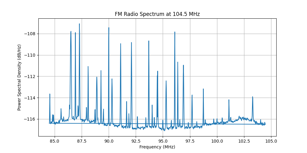
Using the following python code, we can visualise FDM in action by sweeping the FM spectrum:
# Basic FM Spectrum Capture
fromhackrfimport*importmatplotlib.pyplotaspltimportnumpyasnpfromscipy.signalimportwelchwithHackRF()ashrf:hrf.sample_rate=20e6# 20 MHz sample rate
hrf.center_freq=104.5e6# FM Radio
samples=hrf.read_samples(2e6)# Capture 2 million samples
# Compute PSD using Welch’s method (handling complex IQ data)
freqs,psd_values=welch(samples,fs=hrf.sample_rate,nperseg=1024,return_onesided=False)# Convert frequency axis to MHz
freqs_mhz=(freqs-(hrf.sample_rate/2))/1e6+(hrf.center_freq/1e6)# Plot Power Spectral Density
plt.figure(figsize=(10,5))plt.plot(freqs_mhz,10*np.log10(psd_values))# Convert power to dB
plt.xlabel('Frequency (MHz)')plt.ylabel('Power Spectral Density (dB/Hz)')plt.title(f'FM Radio Spectrum at {hrf.center_freq/1e6} MHz')plt.grid()# Save and show
plt.savefig("fm_spectrum.png")plt.show(block=True)
Running this code gave me the following resulting plot (it will be different for you depending on where you live!):
Each sharp peak that you see here represents an FM station at a unique frequency. These are the lanes.
Understanding Modulation
What is Modulation?
Radio signals don’t carry useful information by themselves. Instead, they use modulation to encode voice, music, or
data.
There are two main types of modulation:
Analog Modulation – Used for traditional radio (AM/FM).
Digital Modulation – Used for WiFi, Bluetooth, GPS, and modern systems.
AM (Amplitude Modulation)
AM works by varying the height (amplitude) of the carrier wave to encode audio.
As an example, the carrier frequency stays the same (e.g., 900 kHz), but the amplitude changes based on the sound wave.
AM is prone to static noise (because any electrical interference changes amplitude).
You can capture a sample of AM signals using the hackrf_transfer utility that was installed on your system:
This will capture AM signals at 900 kHz into a file for later analysis.
We can write some python to capture an AM signal and plot the samples so we can visualise this information.
# AM Signal Demodulation
fromhackrfimport*importmatplotlib.pyplotaspltimportnumpyasnpwithHackRF()ashrf:hrf.sample_rate=10e6# 10 MHz sample rate
hrf.center_freq=693e6# 693 MHz AM station
samples=hrf.read_samples(1e6)# Capture 1M samples
# AM Demodulation - Extract Magnitude (Envelope Detection)
demodulated=np.abs(samples)# Plot Demodulated Signal
plt.figure(figsize=(10,5))plt.plot(demodulated[:5000])# Plot first 5000 samples
plt.xlabel("Time")plt.ylabel("Amplitude")plt.title("AM Demodulated Signal")plt.grid()# Save and show
plt.savefig("am_demodulated.png")plt.show(block=True)
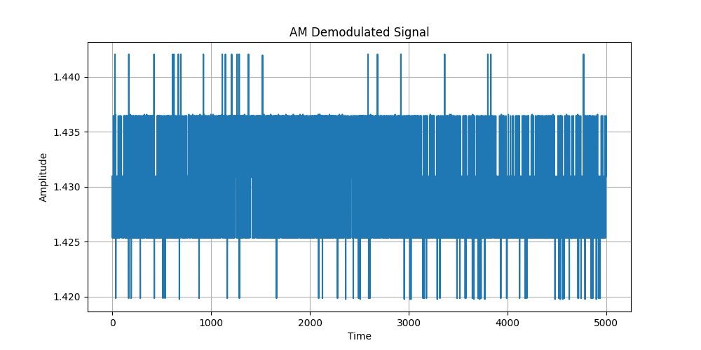
Running this code should give you a plot of what’s happening at 693 MHz:
The plot above represents the amplitude envelope of a real AM radio transmission.
The X-axis represents time, while the Y-axis represents amplitude.
The variations in amplitude correspond to the audio signal encoded by the AM station.
FM (Frequency Modulation)
FM works by varying the frequency of the carrier wave to encode audio.
As an example, the amplitude stays constant, but the frequency changes based on the audio wave.
FM is clearer than AM because it ignores amplitude noise.
You can capture a sample of FM signals with the following:
We can write some python code to capture and demodulate an FM signal as well:
fromhackrfimport*importmatplotlib.pyplotaspltimportnumpyasnpwithHackRF()ashrf:hrf.sample_rate=2e6# 2 MHz sample rate
hrf.center_freq=104.5e6# Example FM station
samples=hrf.read_samples(1e6)# FM Demodulation - Phase Differentiation
phase=np.angle(samples)# Extract phase
fm_demodulated=np.diff(phase)# Differentiate phase
# Plot FM Demodulated Signal
plt.figure(figsize=(10,5))plt.plot(fm_demodulated[:5000])# Plot first 5000 samples
plt.xlabel("Time")plt.ylabel("Frequency Deviation")plt.title("FM Demodulated Signal")plt.grid()# Save and show
plt.savefig("fm_demodulated.png")plt.show(block=True)
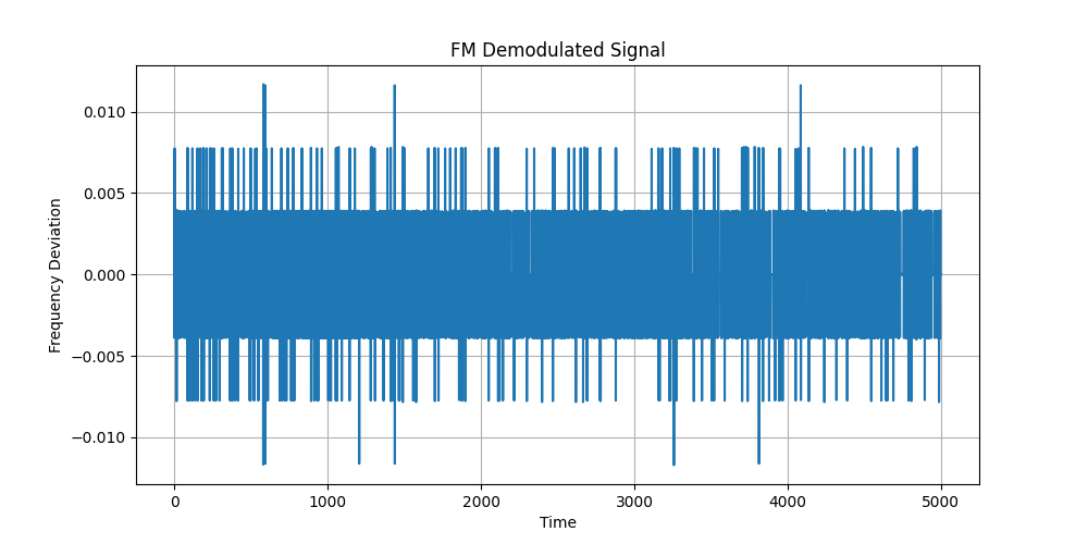
If you pick a frequency that has a local radio station, you should get a strong signal like this:
Unlike AM, where the signal’s amplitude changes, FM signals encode audio by varying the frequency of the carrier wave.
The graph above shows the frequency deviation over time:
The X-axis represents time, showing how the signal changes.
The Y-axis represents frequency deviation, showing how much the carrier frequency shifts.
The spikes and variations represent audio modulation, where frequency shifts encode sound.
If your FM demodulation appears too noisy:
Try tuning to a stronger station (e.g., 100.3 MHz).
Increase the sample rate for a clearer signal.
Apply a low-pass filter to reduce noise in post-processing.
Bandwidth of a Modulated Signal
Modulated signals require bandwidth (\(B\)), and the amount depends on the modulation type.
AM
The total bandwidth required for AM signals is:
\[B = 2f_m\]
Where:
\(B\) = Bandwidth in Hz
\(f_m\) = Maximum audio modulation frequency in Hz
If an AM station transmits audio up to 5 kHz, the bandwidth is:
\[B = 2 \times 5\text{kHz} = 10\text{kHz}\]
This explains why AM radio stations typically require ~10 kHz per station.
FM
The bandwidth required for an FM signal follows Carson’s Rule:
\[B = 2 (f_d + f_m)\]
Where:
\(f_d\) = Peak frequency deviation (how much the frequency shifts)
\(f_m\) = Maximum audio frequency in Hz
For an FM station with a deviation of 75 kHz and max audio frequency of 15 kHz, the total bandwidth is:
\[B = 2 (75 + 15) = 180 \text{kHz}\]
This explains why FM radio stations require much more bandwidth (~200 kHz per station).
Digital Modulation
For digital signals, it’s important to be able to transmit binary data (1’s and 0’s). These methods of modulation are
focused on making this process much more optimal than what the analog counterparts could provide.
What is FSK (Frequency Shift Keying)?
FSK is digital FM—instead of smoothly varying frequency like FM radio, it switches between two frequencies for 0’s and
1’s. This method of modulation is used in technologies like Bluetooth, LoRa, and old-school modems.
Example:
A “0” might be transmitted as a lower frequency (e.g., 915 MHz).
A “1” might be transmitted as a higher frequency (e.g., 917 MHz).
The receiver detects these frequency changes and reconstructs the binary data.
What is PSK (Phase Shift Keying)?
PSK is digital AM—instead of changing amplitude, it shifts the phase of the wave. This method of modulation is used
in technologies like WiFi, GPS, 4G LTE, Satellites.
Example:
0° phase shift = Binary 0
180° phase shift = Binary 1
More advanced PSK (like QPSK) uses four phase shifts (0°, 90°, 180°, 270°) to send two bits per symbol (faster data transmission).
Wrapping Up
In this post, we explored the fundamentals of radio signals—what they are, how they work, and how different modulation
techniques like AM and FM allow signals to carry audio through the air.
This really is only the start of what you can get done with software defined radio. Here are some further resources to
check out: