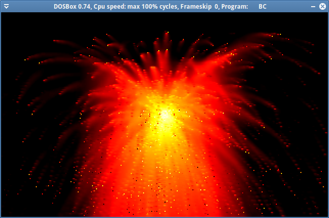
Time to do another write up on an old demo effect that’s always a crowd pleaser. A particle system. In today’s post, this particle system will act like a geyser of pixels acting under gravity that will appear to burn as the tumble down the screen.
We’re working in old school mode 13 (320x200x256) today in DOS.
Trust me. It looks a lot more impressive when it’s animating!
The envrionment
First of all, we’ll start off by defining some global, environment level constants that will control the simulation for us. It’s always good to define this information as constants as it allows for quick tweaking.
#define PARTICLE_COUNT		1000
#define GRAVITY				0.1f
PARTICLE_COUNT will control the number of particles in total for our simulation and GRAVITY controls the amount of pull on the y-axis that the particles will experience whilst they’re in the simulation.
Next, we need to define the particles themselves.
What’s a particle
The data that makes up a particle is a position (x and y), a velocity (vx and vy), life and decay. The velocity variables (vx and vy) impact the position variables (x and y) after each frame of animation. The GRAVITY constant impatcs the y velocity (vy) in such a way that all particles are biased towards the bottom of the screen over time. The decay variable is used to determine how much life is lost from the particle per frame and finally life itself determines how far through the colour scale that the particle should be drawn.
The life variable is tightly related to the way that we setup our indexed palette also. With life starting at 255.0f; making its way to 0.0f we interpolate its value over a 255..0 range so that it can directly correspond to a colour index. The way the colour index is setup, a particle at its strongest life will be white; it’ll move its way through yellow, orange to red finally ending at black (which will be 0).
From these variables (per particle) we can animate its rather short-life on screen. We can easily wrap all of this information up into a structure:
There are some default actions that we need to define for these particles though. We really need a way to initialise, render and update them in order to animate their characteristics appropriately.
All of the functions that are written for this particle system operate on an array index. The array itself is globally defined.
Initialisation is just setting some starting values for the particle. You can play with these values to taste, but I personally like a random velocity (in any direction):
As I said above, we’re in mode 13. We’ve got 320x200 pixels to work with, so I start all particles off in the centre of the screen. Velocities are set using the standard random number generator inside of libc. life starts at the top of the spectrum and decay is defined very, very close to 1.0f.
Rendering a particle is dead-simple. We just draw a pixel on the screen.
The position is augmented by the velocity, the y velocity by the gravity and life by the decay. vx is also adjusted by multiplication of a constant very close to 1.0f. This is just to dampen the particle’s spread on the x-axis.
Finally, if a particle has move outside of its renderable environment or it’s dead we just re-initialize it.
The secret sauce
If this is where we left the simulation, it’d look pretty sucky. Not only would we just have a fountain of pixels, but nothing would really appear to animate as your screen filled up with pixelated arcs following the colour palette spectrum that’d been setup.
We average the colour of the pixels on screen to give the particle system a glow (or bloom). This also works well with not clearing the screen before every re-draw as we want the trails of the particles left around so that they’ll appear to burn up.
Direct access to video memory through assembly language allows us to get this done in a nice, tight loop:
In today’s post, I’m just going to gloss over some top level details in developing applications that use Berkeley DB.
What is it?
The first line of the Wikipedia article for Berkeley DB sums the whole story up pretty well, I think:
Berkeley DB (BDB) is a software library that provides a high-performance embedded database for key/value data.
Pretty simple. Berkeley DB is going to offer you an in-process database to manage data in your applications in a little more organised approach.
Getting installed
I’m using Debian Linux, more specifically the testing release. I’m sure the installation process will translate for other Debian releases and/or other Linux distributions with their respective package managers.
If you’ve already got a standard development/build environment running, you won’t need the build-essential package listed below.
sudo apt-get install build-essential libdb-dev
Building applications
Once you’ve finished writing an application using this library, you’ll need to link the Berkeley DB library against your application. This is all pretty simple as well:
gcc -ldb yourapp.o -o yourapp
The key piece being the -ldb linker library switch.
Some simple operations
The following blocks of code are heavily based off of the information contained in this pdf. That pdf has a heap of information in it well worth the read if you’re going to do something serious with Berkeley DB.
First thing you need to do, is to initialize the database structure that you’ll use to conduct all of your operations.
DB*db;intret;/* setup the database memory structure */ret=db_create(&db,NULL,0);
db_create will allocate and fill out the structure of the DB typed pointer. It just sets it up ready for use. Once you’ve created the database handle, it’s time to actually open up a database (or create one).
open is going to try and find the requested database; (in my case test.db) and open it up. Failing that, it’ll create it (because of DB_CREATE). The format parameter is quite interesting. In the sample above, DB_BTREE has been specified. Looking at the DB->open() documentation:
The currently supported Berkeley DB file formats (or access methods) are Btree, Hash, Queue, and Recno. The Btree format is a representation of a sorted, balanced tree structure. The Hash format is an extensible, dynamic hashing scheme. The Queue format supports fast access to fixed-length records accessed sequentially or by logical record number. The Recno format supports fixed- or variable-length records, accessed sequentially or by logical record number, and optionally backed by a flat text file.
This gives you the flexability to use the format that suits your application best.
Once the database is open, writing data into it is as easy as specifying a key and value. There are some further data structures that need to be filled out, but the code is pretty easy to follow:
/* source data values */char*name="John Smith";intid=5;DBTkey,value;memset(&key,0,sizeof(DBT));memset(&value,0,sizeof(DBT));/* setup the key */key.data=&id;key.size=sizeof(int);/* setup the value */value.data=name;value.size=strlen(name)+1;/* write it into the database */ret=db->put(db,NULL,&key,&value,DB_NOOVERWRITE);
As the data member of the DBT struct is typed out as void *, you can store any information you’d like in there. Of course, you must specify the size so the system knows how much to write.
Reading values back out into native variables is just as easy:
/* destinations */charread_name[256];intread_id=5;memset(&key,0,sizeof(DBT));memset(&value,0,sizeof(DBT));/* setup the key to read */key.data=&read_id;key.size=sizeof(int);/* setup the value to fill */value.data=read_name;value.ulen=256;value.flags=DB_DBT_USERMEM;db->get(db,NULL,&key,&value,0);
Finally, you’ll want to close your database once you’re done:
The installation itself is pretty straight forward, however there is a little bit of reconfig work and user administration to get going for non-root users.
Install Wireshark from apt
$ sudo apt-get install wireshark
Reconfigure the wireshark-common package making sure to answer yes to the question asked.
$ sudo dpkg-reconfigure wireshark-common
Add any user to the wireshark group that needs to be able to capture data off the network interfaces.
$ sudo usermod -a-G wireshark $USER
Remember, if you added yourself to this group; you’ll need to logout and log back in for the group changes to take effect.
If you’re on a fresh machine, and you’re downloading/installing Eclipse for the purposes of Java development, you’ll want to install the JDK. To get this going, I install the openjdk-7-jdk out of the apt repository.
$ sudo apt-get install openjdk-7-jdk
After that finishes, or while, grab a copy of the Eclipse version that you need from the download page. Once it’s down, I normally extract it and then put it in a system-wide location (as opposed to just running it from my home directory).
Taking your applications from the development web server into a full application server environment is quite painless with nginx, uwsgi and virtualenv. This post will take you through the steps required to get an application deployed.
Server Setup
First of all, you’ll need to get your server in a state where it’s capable of serving HTTP content as well as housing your applications. If you’ve already got a server that will do this, you can skip this.
This will put all of the software required onto the server to house these applications.
Application setup with uWSGI
Each uWSGI application’s configuration is represented on the filesystem as an ini file, typically found in /etc/uwsgi/apps-available. Symlinks are established between files in this directory into /etc/uwsgi/apps-enabled to tell the uwsgi daemon that an application needs to be running.
The following is an example uWSGI configuration file that you can use as a template:
This will get our application housed by uWSGI. You can now enable this application:
$ sudo ln-s /etc/uwsgi/apps-available/app.ini /etc/uwsgi/apps-enabled/app.ini
$ sudo service uwsgi restart
Web server setup
Finally, we’ll get nginx to provide web access to our application. You may have specific web site files that you need to modify to do this, but this example assumes that you’re in control of the default application.
Add the following section to /etc/nginx/sites-available/default: