Exploring Advanced Word Embeddings
20 Oct 2024Introduction
In our previous posts, we explored traditional text representation techniques like One-Hot Encoding, Bag-of-Words, and TF-IDF, and we introduced static word embeddings like Word2Vec and GloVe. While these techniques are powerful, they have limitations, especially when it comes to capturing the context of words.
In this post, we’ll explore more advanced topics that push the boundaries of NLP:
- Contextual Word Embeddings like ELMo, BERT, and GPT
- Dimensionality Reduction techniques for visualizing embeddings
- Applications of Word Embeddings in real-world tasks
- Training Custom Word Embeddings on your own data
Let’s dive in!
Contextual Word Embeddings
Traditional embeddings like Word2Vec and GloVe generate a single fixed vector for each word. This means the word “bank” will have the same vector whether it refers to a “river bank” or a “financial institution,” which is a major limitation in understanding nuanced meanings in context.
Contextual embeddings, on the other hand, generate different vectors for the same word depending on its context. These models are based on deep learning architectures and have revolutionized NLP by capturing the dynamic nature of language.
ELMo (Embeddings from Language Models)
ELMo was one of the first models to introduce the idea of context-dependent word representations. Instead of a fixed vector, ELMo generates a vector for each word that depends on the entire sentence. It uses bidirectional LSTMs to achieve this, looking both forward and backward in the text to understand the context.
BERT (Bidirectional Encoder Representations from Transformers)
BERT takes contextual embeddings to the next level using the Transformer architecture. Unlike traditional models, which process text in one direction (left-to-right or right-to-left), BERT is bidirectional, meaning it looks at all the words before and after a given word to understand its meaning. BERT also uses pretraining and fine-tuning, making it one of the most versatile models in NLP.
GPT (Generative Pretrained Transformer)
While GPT is similar to BERT in using the Transformer architecture, it is primarily unidirectional and excels at generating text. This model has been the backbone for many state-of-the-art systems in tasks like text generation, summarization, and dialogue systems.
Why Contextual Embeddings Matter
Contextual embeddings are critical in modern NLP applications, such as:
- Named Entity Recognition (NER): Contextual models help disambiguate words with multiple meanings.
- Machine Translation: These embeddings capture the nuances of language, making translations more accurate.
- Question-Answering: Systems like GPT-3 excel in understanding and responding to complex queries by leveraging context.
To experiment with BERT, you can try the transformers library from Hugging Face:
from transformers import BertTokenizer, BertModel

# Load pre-trained model tokenizer
tokenizer = BertTokenizer.from_pretrained('bert-base-uncased')

# Tokenize input text
text = "NLP is amazing!"
encoded_input = tokenizer(text, return_tensors='pt')

# Load pre-trained BERT model
model = BertModel.from_pretrained('bert-base-uncased')

# Get word embeddings from BERT
output = model(**encoded_input)
print(output.last_hidden_state)
The tensor output from this process should look something like this:
tensor([[[ 0.0762,  0.0177,  0.0297,  ..., -0.2109,  0.2140,  0.3130],
         [ 0.1237, -1.0247,  0.6718,  ..., -0.3978,  0.9643,  0.7842],
         [-0.2696, -0.3281,  0.3901,  ..., -0.4611, -0.3425,  0.2534],
         ...,
         [ 0.2051,  0.2455, -0.1299,  ..., -0.3859,  0.1110, -0.4565],
         [-0.0241, -0.7068, -0.4130,  ...,  0.9138,  0.3254, -0.5250],
         [ 0.7112,  0.0574, -0.2164,  ...,  0.2193, -0.7162, -0.1466]]],
    grad_fn=<NativeLayerNormBackward0>)
2. Visualizing Word Embeddings
Word embeddings are usually represented as high-dimensional vectors (e.g., 300 dimensions for Word2Vec). While this is great for models, it’s difficult for humans to interpret these vectors directly. This is where dimensionality reduction techniques like PCA and t-SNE come in handy.
Principal Component Analysis (PCA)
PCA reduces the dimensions of the word vectors while preserving the most important information. It helps us visualize clusters of similar words in a lower-dimensional space (e.g., 2D or 3D).
Following on from the previous example, we’ll use the simple embeddings that we’ve generated in the output variable.
from sklearn.decomposition import PCA
import matplotlib.pyplot as plt

# . . .

embeddings = output.last_hidden_state.detach().numpy()

# Reduce embeddings dimensionality with PCA
# The embeddings are 3D (1, sequence_length, hidden_size), so we flatten the first two dimensions
embeddings_2d = embeddings[0]  # Remove the batch dimension, now (sequence_length, hidden_size)

# Apply PCA
pca = PCA(n_components=2)
reduced_embeddings = pca.fit_transform(embeddings_2d)

# Visualize the first two principal components of each token's embedding
plt.figure(figsize=(8,6))
plt.scatter(reduced_embeddings[:, 0], reduced_embeddings[:, 1])

# Add labels for each token
tokens = tokenizer.convert_ids_to_tokens(encoded_input['input_ids'][0])
for i, token in enumerate(tokens):
plt.annotate(token, (reduced_embeddings[i, 0], reduced_embeddings[i, 1]))

plt.title('PCA of BERT Token Embeddings')
plt.xlabel('Principal Component 1')
plt.ylabel('Principal Component 2')
plt.savefig('bert_token_embeddings_pca.png', format='png')
You should see a plot similar to this:
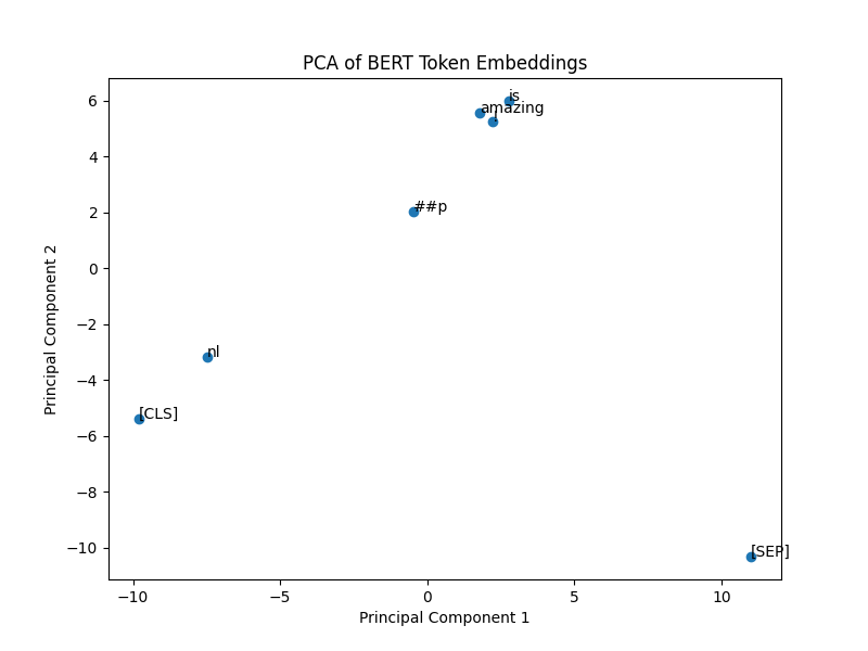
This is a scatter plot where the 768 dimensions of each embedding has been reduced two to 2 principal components using Principal Component Analysis (PCA). This allows us to plot these in two-dimensional space.
Some observations when looking at this chart:
Special Tokens [CLS] and [SEP]
These special tokens are essential in BERT. The [CLS] token is typically used as a summary representation for the
entire sentence (especially in classification tasks), and the [SEP] token is used to separate sentences or indicate
the end of a sentence.
In the plot, you can see [CLS] and [SEP] are far apart from other tokens, especially [SEP], which has a distinct
position in the vector space. This makes sense since their roles are unique compared to actual word tokens like “amazing”
or “is.”
Subword Tokens
Notice the token labeled ##p. This represents a subword. BERT uses a WordPiece tokenization algorithm, which
breaks rare or complex words into subword units. In this case, “NLP” has been split into nl and ##p because BERT
doesn’t have “NLP” as a whole word in its vocabulary. The fact that nl and ##p are close together in the plot
indicates that BERT keeps semantically related parts of the same word close in the vector space.
Contextual Similarity
The tokens “amazing” and “is” are relatively close to each other, which reflects that they are part of the same sentence and share a contextual relationship. Interestingly, “amazing” is a bit more isolated, which could be because it’s a more distinctive word with a strong meaning, whereas “is” is a more common auxiliary verb and closer to other less distinctive tokens.
Distribution and Separation
The distance between tokens shows how BERT separates different tokens in the vector space based on their contextual
meaning. For example, [SEP] is far from the other tokens because it serves a very different role in the sentence.
The overall spread of the tokens suggests that BERT embeddings can clearly distinguish between different word types
(subwords, regular words, and special tokens).
t-SNE (t-Distributed Stochastic Neighbor Embedding)
t-SNE is another popular technique for visualizing high-dimensional data. It captures both local and global structures of the embeddings and is often used to visualize word clusters based on their semantic similarity.
I’ve continued on from the code that we’ve been using:
from sklearn.manifold import TSNE
import matplotlib.pyplot as plt

embeddings = output.last_hidden_state.detach().numpy()[0]

# use TSNE here
tsne = TSNE(n_components=2, random_state=42, perplexity=1)
reduced_embeddings = tsne.fit_transform(embeddings)

# Plot the t-SNE reduced embeddings
plt.figure(figsize=(8, 6))
plt.scatter(reduced_embeddings[:, 0], reduced_embeddings[:, 1])

# Add labels for each token
for i, token in enumerate(tokens):
plt.annotate(token, (reduced_embeddings[i, 0], reduced_embeddings[i, 1]))

plt.title('t-SNE of BERT Token Embeddings')
plt.xlabel('Dimension 1')
plt.ylabel('Dimension 2')

# Save the plot to a file
plt.savefig('bert_token_embeddings_tsne.png', format='png')
The output of which looks a little different to PCA:
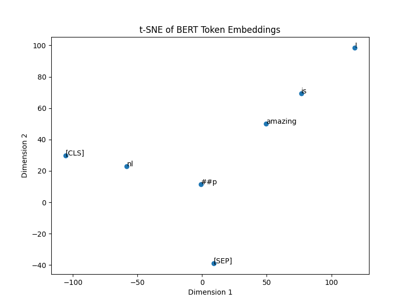
There is a different distribution of the embeddings in comparison.
Real-World Applications of Word Embeddings
Word embeddings are foundational in numerous NLP applications:
- Semantic Search: Embeddings allow search engines to find documents based on meaning rather than exact keyword matches.
- Sentiment Analysis: Embeddings can capture the sentiment of text, enabling models to predict whether a review is positive or negative.
- Machine Translation: By representing words from different languages in the same space, embeddings improve the accuracy of machine translation systems.
- Question-Answering Systems: Modern systems like GPT-3 use embeddings to understand and respond to natural language queries.
Example: Semantic Search with Word Embeddings
In a semantic search engine, user queries and documents are both represented as vectors in the same embedding space. By calculating the cosine similarity between these vectors, we can retrieve documents that are semantically related to the query.
import numpy as np
from sklearn.metrics.pairwise import cosine_similarity

# Simulate a query embedding (1D vector of size 768, similar to BERT output)
query_embedding = np.random.rand(1, 768)  # Shape: (1, 768)

# Simulate a set of 5 document embeddings (5 documents, each with a 768-dimensional vector)
document_embeddings = np.random.rand(5, 768)  # Shape: (5, 768)

# Compute cosine similarity between the query and the documents
similarities = cosine_similarity(query_embedding, document_embeddings)  # Shape: (1, 5)

# Rank documents by similarity (higher similarity first)
ranked_indices = similarities.argsort()[0][::-1]  # Sort in descending order
print("Ranked document indices (most similar to least similar):", ranked_indices)

# If you want to print the similarity scores as well
print("Similarity scores:", similarities[0][ranked_indices])
Walking through this code:
query_embedding and document_embeddings
-
We generate random vectors to simulate the embeddings. In a real use case, these would come from an embedding model (e.g., BERT, Word2Vec). The
query_embeddingrepresents the vector for the user’s query, anddocument_embeddingsrepresents vectors for a set of documents. -
Both
query_embeddinganddocument_embeddingsmust have the same dimensionality (e.g., 768 if you’re using BERT).
Cosine Similarity
- The
cosine_similarity()function computes the cosine similarity between thequery_embeddingand each document embedding. - Cosine similarity measures the cosine of the angle between two vectors, which ranges from -1 (completely dissimilar) to 1 (completely similar). In this case, we’re interested in documents that are most similar to the query (values close to 1).
Ranking the Documents
- We use
argsort()to get the indices of the document embeddings sorted in ascending order of similarity. - The
[::-1]reverses this order so that the most similar documents appear first. - The
ranked_indicesgives the document indices, ranked from most similar to least similar to the query.
The output of which looks like this:
Ranked document indices (most similar to least similar): [3 4 1 2 0]
Similarity scores: [0.76979867 0.7686247  0.75195574 0.74263041 0.72975817]
Training Your Own Word Embeddings
While pretrained embeddings like Word2Vec and BERT are incredibly powerful, sometimes you need embeddings that are fine-tuned to your specific domain or dataset. You can train your own embeddings using frameworks like Gensim for Word2Vec or PyTorch for more complex models.
The following code shows training Word2Vec with Gensim:
from gensim.models import Word2Vec
import nltk
from nltk.tokenize import word_tokenize

nltk.download('punkt_tab')

# Example sentences
sentences = [
    word_tokenize("I love NLP"),
    word_tokenize("NLP is amazing"),
    word_tokenize("Word embeddings are cool")
]

# Train Word2Vec model
model = Word2Vec(sentences, vector_size=100, window=5, min_count=1, workers=4)
# Get vector for a word
vector = model.wv['NLP']
print(vector)
The output here is a 100-dimensional vector that represents the word NLP.
[-5.3622725e-04  2.3643136e-04  5.1033497e-03  9.0092728e-03
 -9.3029495e-03 -7.1168090e-03  6.4588725e-03  8.9729885e-03

  . . . . . .

  . . . . . .

 3.4736372e-03  2.1777749e-04  9.6188262e-03  5.0606038e-03
 -8.9173904e-03 -7.0415605e-03  9.0145587e-04  6.3925339e-03]
Fine-Tuning BERT with PyTorch
You can also fine-tune BERT or other transformer models on your own dataset. This is useful when you need embeddings that are tailored to a specific domain, such as medical or legal text.
Conclusion
Word embeddings have come a long way, from static models like Word2Vec and GloVe to dynamic, context-aware models like BERT and GPT. These techniques have revolutionized how we represent and process language in NLP. Alongside dimensionality reduction for visualization, applications such as semantic search, sentiment analysis, and custom embeddings training open up a world of possibilities.